support@comsol.com
Wave Optics Module Updates
For users of the Wave Optics Module, COMSOL Multiphysics® version 6.2 introduces performance improvements to the Electromagnetic Waves, Boundary Elements interface, new impedance boundary conditions, and a tutorial model that describes wave propagation in liquid crystals. Learn more about these updates below.
Performance Improvements for the Electromagnetic Waves, Boundary Elements Interface
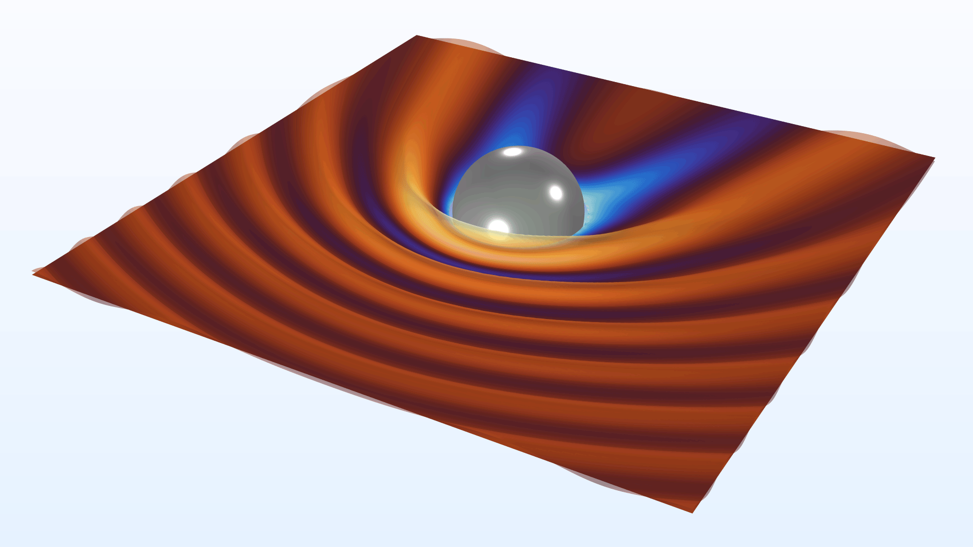
In the settings for the Electromagnetic Waves, Boundary Elements interface, it is now possible to select symmetry planes to reduce computation time. The symmetry settings also control the far-field calculations and the physics-controlled meshing. The new RCS of a Metallic Sphere Using the Boundary Element Method (RF) model showcases this functionality.
Furthermore, boundary element method (BEM) simulations on clusters are up to 2.5 times faster than in previous versions. If you also include the effect of reducing the model using a symmetry plane, then the simulation times are up to 4 times faster. Additionally, the load and memory balancing for BEM models running on clusters has been significantly improved.
New and Improved Features in the Electromagnetic Waves, Boundary Elements Interface
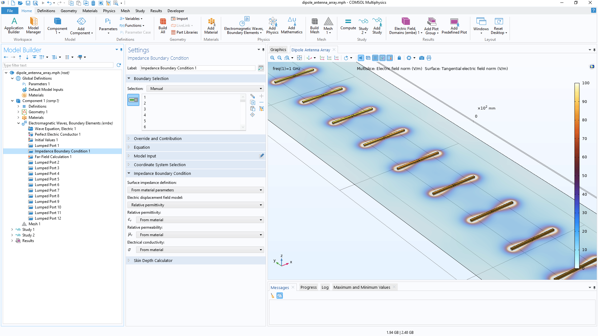
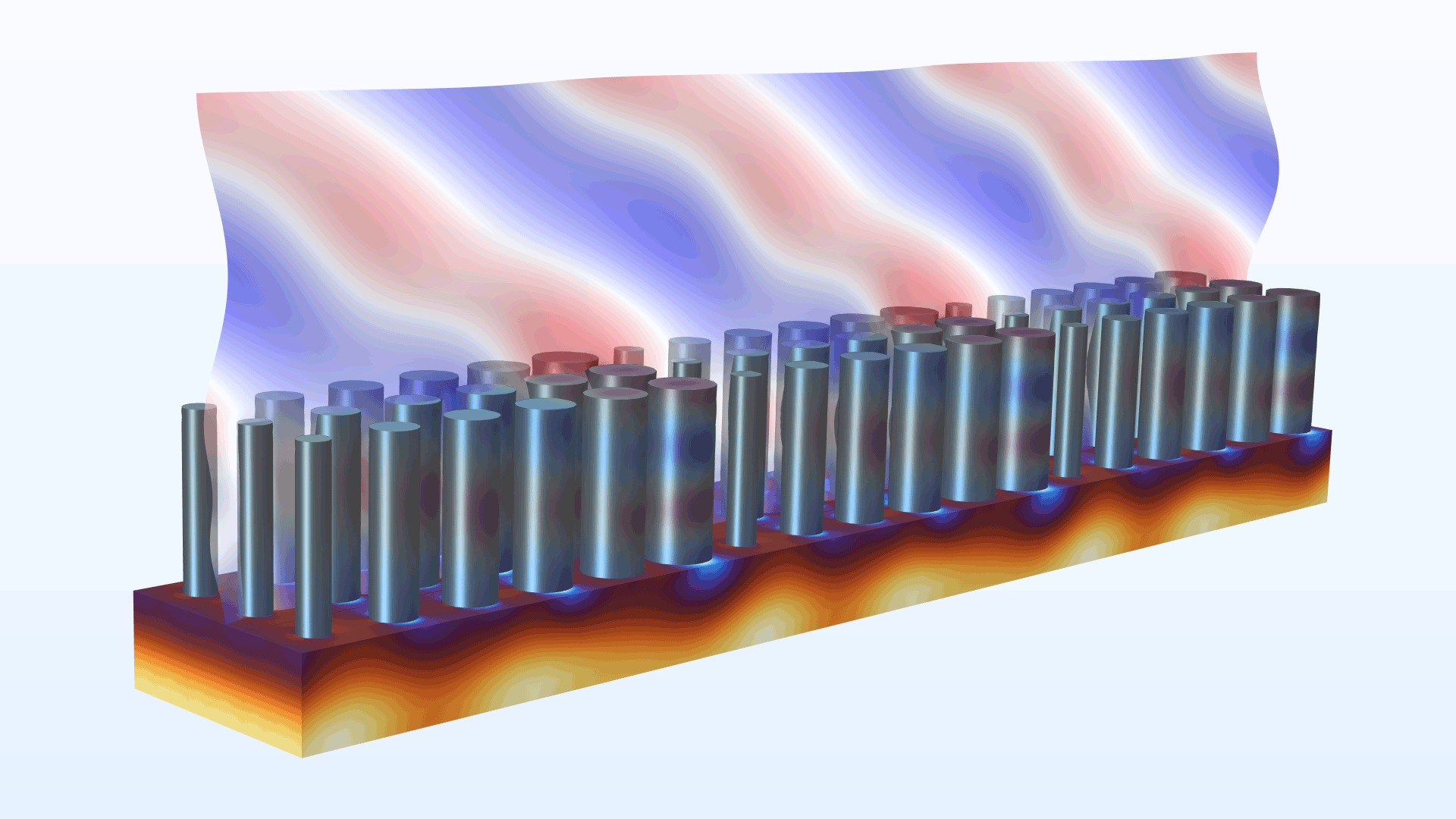
The Impedance Boundary Condition and the Layered Impedance Boundary Condition have been added to the Electromagnetic Waves, Boundary Elements interface. These boundary conditions handle metallic exterior domains and metallic exterior domains covered by a layer structure, respectively. You can view this new addition in the Modeling of Dipole Antenna Array Using the Boundary Element Method tutorial model.
The default feature, Wave Equation, Electric, now includes all standard Electric displacement field model options, such as Relative permittivity, Refractive index, Dielectric loss, etc. This simplifies the use of different materials, supporting different material models.
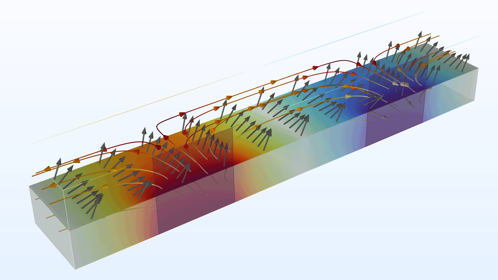
Wave Propagation Through Liquid Crystals
A new tutorial model demonstrates the switching capability of a liquid-crystal (LC) display cell in an in-plane switching (IPS) configuration. The Oseen–Frank model is used to solve for the LC director (optical axis) distribution when a static electric field is applied. An equation-based interface is used to define the Oseen–Frank equation, whereas the Electrostatics interface is used to solve for the electric potential distribution. For the given inhomogeneous anisotropic LC material, a full-wave simulation is performed using the Electromagnetic Waves, Frequency Domain interface.
Incident Wave Direction Input Field for Gaussian Beams
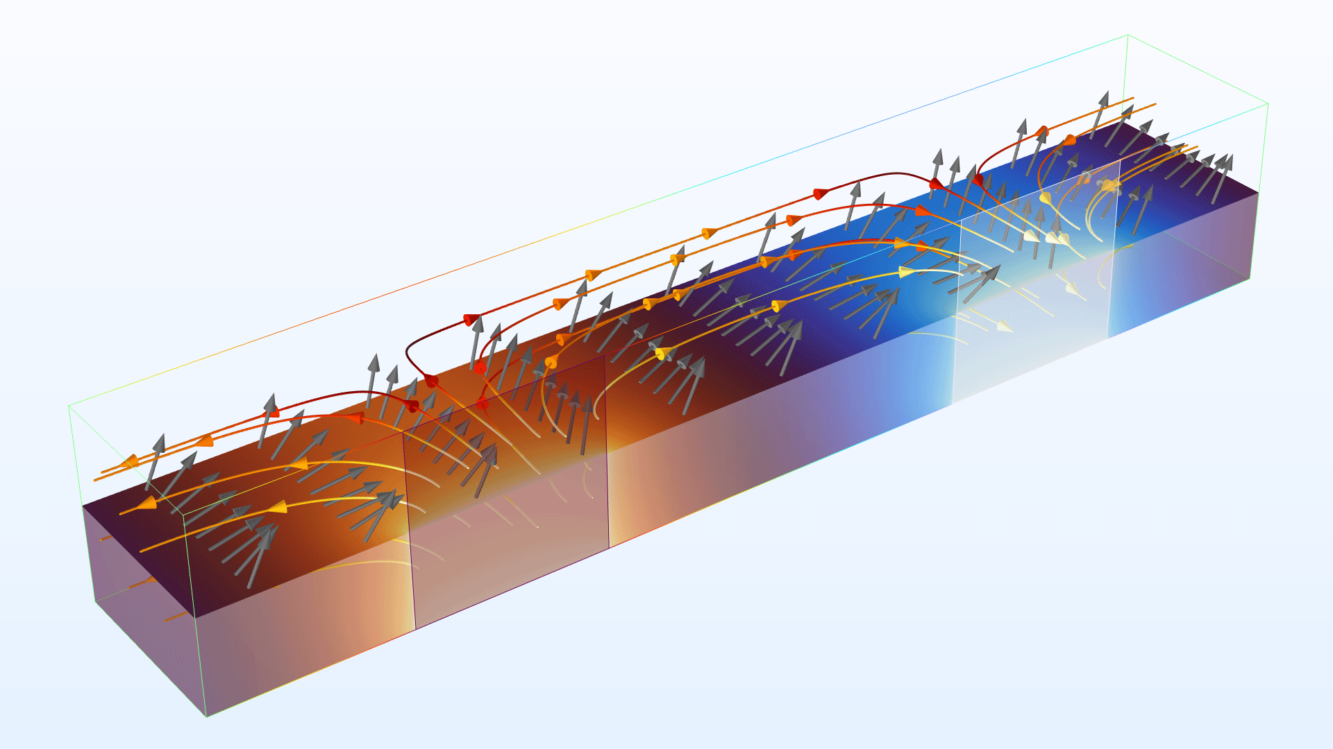
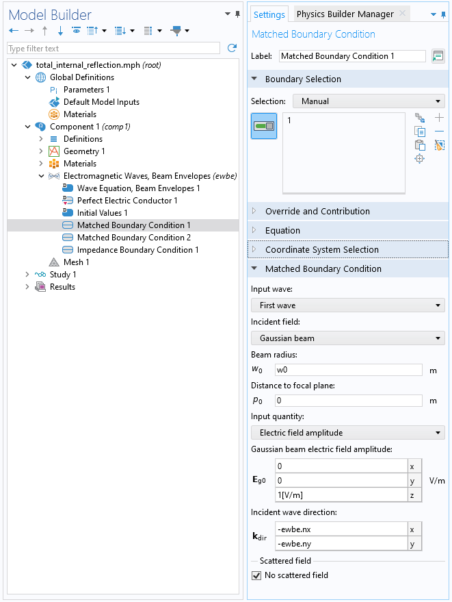
When using the Gaussian beam input option in the Scattering Boundary Condition and Matched Boundary Condition features in the Electromagnetic Waves, Beam Envelopes interface, there is a new Incident wave direction input field. This input field specifies the main propagation direction for the incident Gaussian beam, enabling greater flexibility when specifying Gaussian input beams with complex inhomogeneous wave-vector distributions on the interface node.
Electrical Conductivity Added to Drude–Lorentz and Debye Dispersion Models
The Drude–Lorentz and Debye dispersion models now have additional flexibility, allowing separate input of the electrical conductivity.
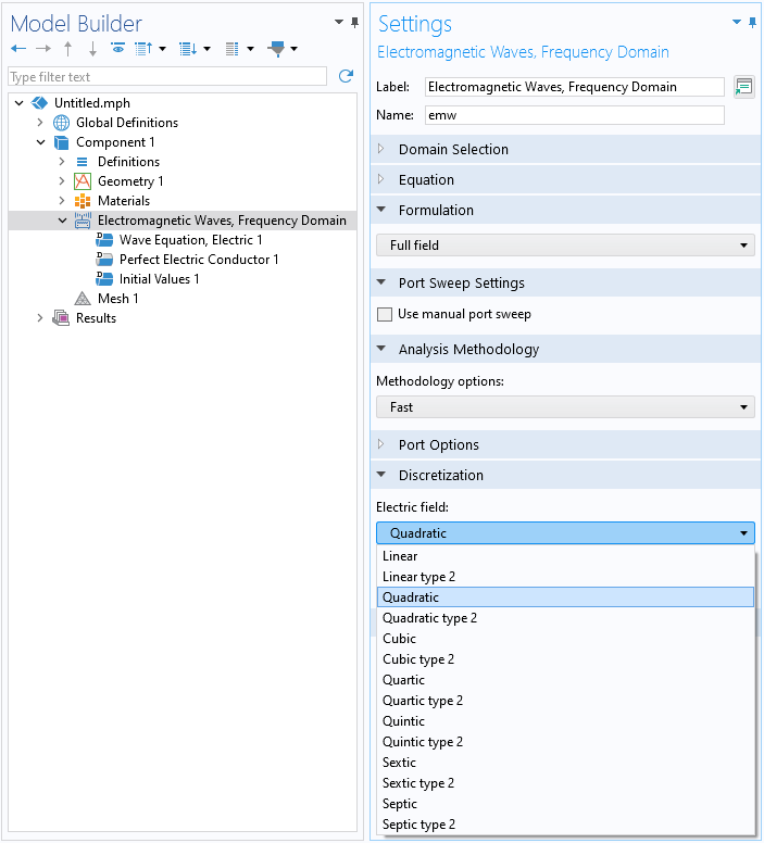
Higher-Order Elements
In this version, up to seventh-order curl elements can now be used in the Electromagnetic Waves, Frequency Domain interface and the Electromagnetic Waves, Transient interface.
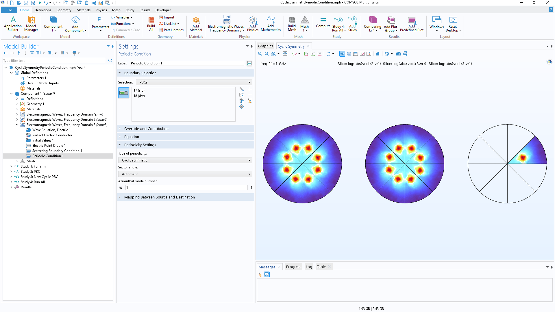
Cyclic Symmetry for Periodic Condition
Cyclic symmetry has been added as a periodicity option for the Periodic Condition feature. This option provides the ability to perform simulations of one sector of a full, cyclically symmetric model as opposed to the full model, reducing computation time.
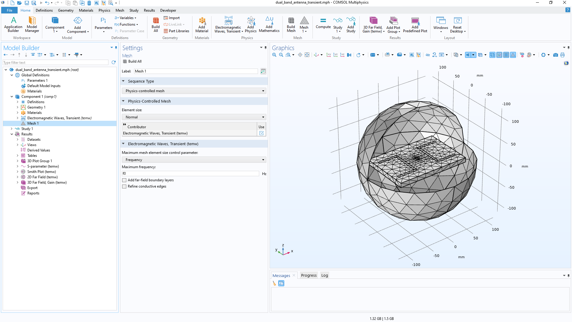
Time-Domain Physics-Controlled Mesh
The time-domain interfaces, Electromagnetic Waves, Transient and Electromagnetic Waves, Time Explicit, now provide physics-controlled mesh suggestions based on the frequency or wavelength content of a simulation. The following tutorial models showcase this new update:
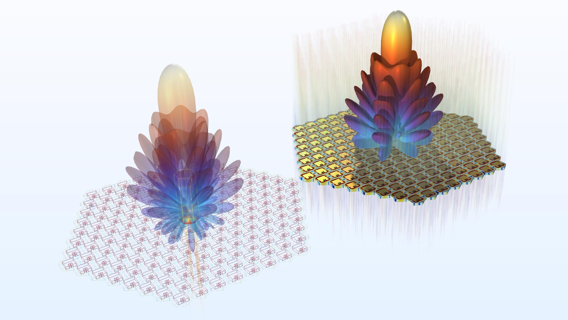
Hexagonal Uniform Array Factor
The hexagonal uniform array factor quickly estimates the far-field pattern of antenna arrays on a triangular grid. In version 6.2, the hexagonal antenna arrays provide lower sidelobes, more robust performance with better resolution, lower spatial noise, and wider coverage.
Instantaneous Norm Variables for Vector Quantities
There are new variables that can be added to the form phys.normXi = sqrt(real(Xx)^2+real(Xy)^2+real(Xz)^2), where phys is a placeholder for any physics tag, such as ewfd, and X is a placeholder for a physical quantity, such as an electric field (E), magnetic field (H), etc. These variables are especially useful when visualizing time-harmonic vector waves.
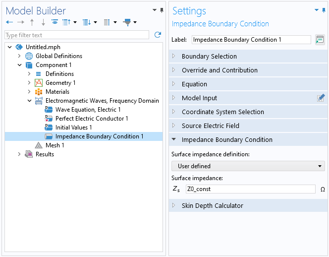
User-Defined Surface Impedance
In the Impedance Boundary Condition feature and the Layered Impedance Boundary Condition feature, it is now possible to directly enter a surface impedance. Previously, the surface impedance was calculated indirectly from the material properties defined on the boundary or in the feature settings. This simplifies the modeling process for problems where it is less relevant to use actual materials for modeling the exterior domain.
Optical Material Library Updates
Within the Optical material library, available in the Ray Optics Module and the Wave Optics Module, more than 90 new glasses from CDGM Glass Co., Ltd. have been added. The new glasses contain all of the necessary properties to perform structural-thermal-optical performance (STOP) analysis.
New Tutorial Models
COMSOL Multiphysics® version 6.2 brings the following new tutorial models to the Wave Optics Module.
In-Plane Switching of a Liquid Crystal Cell
Application Library Title:
in_plane_switching_liquid_crystal_cell
Download from the Application Gallery
Metasurface Beam Deflector
Application Library Title:
metasurface_beam_deflector
Download from the Application Gallery
RCS of a Metallic Sphere Using the Boundary Element Method
Application Library Title:
rcs_sphere_bem
Download from the Application Gallery
Simulation of Metal–Air Surface Plasmon Polariton Propagation and Dispersion
Application Library Title:
metal_air_surface_plasmon_polariton
Download from the Application Gallery
Waveguide S-Bend

Application Library Title:
waveguide_s_bend
Download from the Application Gallery