support@comsol.com
CFD Module Updates
For users of the CFD Module, COMSOL Multiphysics® version 6.1 provides a new Detached Eddy Simulation interface, the ability to use Reynolds-averaged Navier–Stokes (RANS) turbulence models in porous domains, and interfaces for modeling chemical species transport and reactions in combination with high Mach number flow. Read more about the CFD updates below.
Detached Eddy Simulation Interface
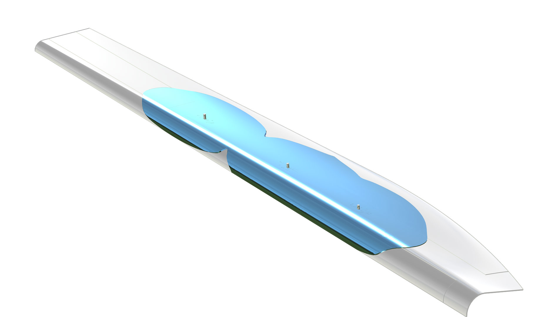
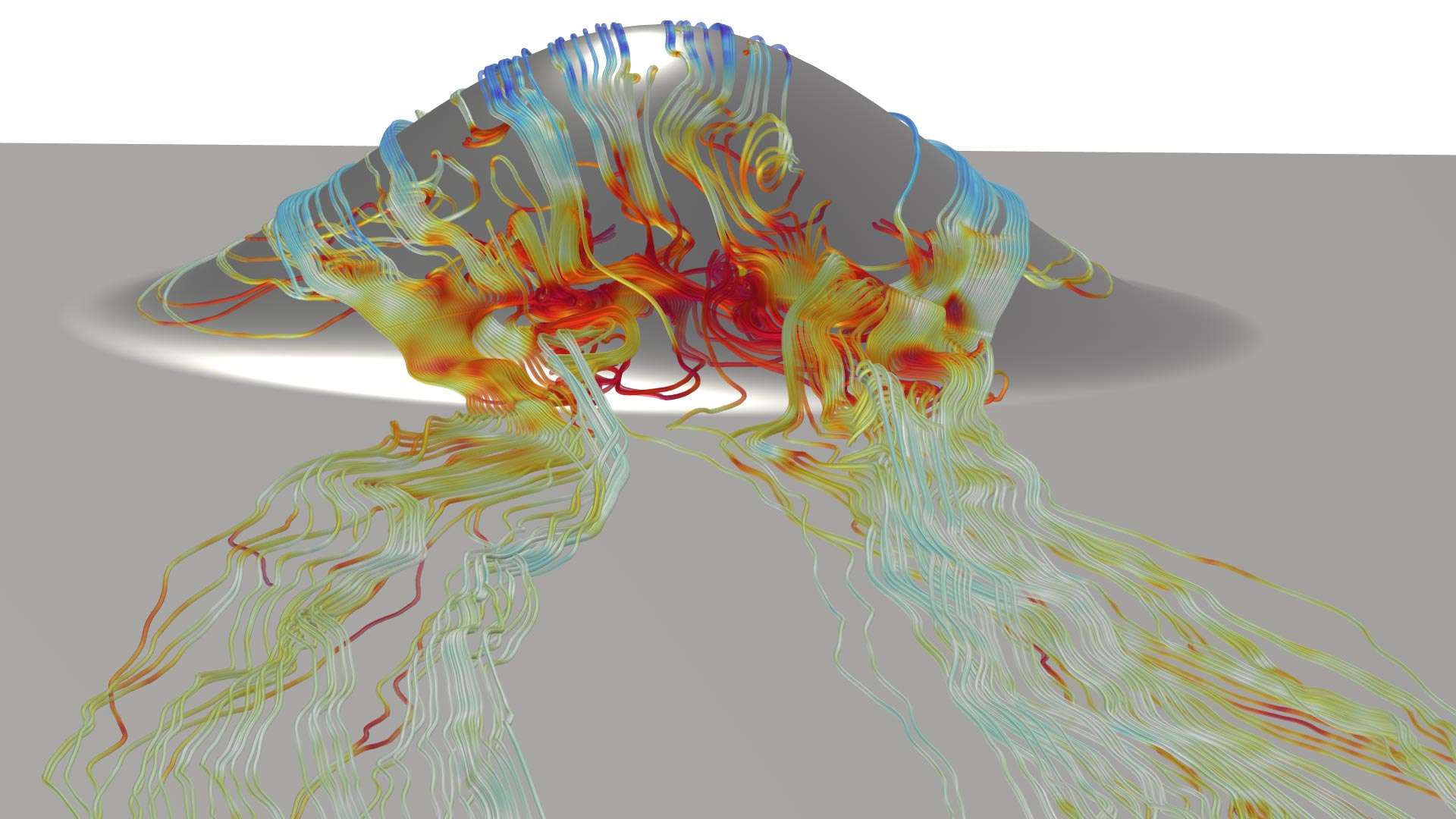
A new Detached Eddy Simulation (DES) interface formulates a hybrid method between RANS and large eddy simulation (LES), where RANS is used in the boundary layer and LES is used elsewhere. The benefit of this method is that it requires a less dense boundary layer mesh compared with a pure LES. This substantially reduces the memory requirement and computation time when the model equations are being solved. For some cases, this improved computational performance is achieved with only a minor impact on accuracy. The DES interface combines the Spalart–Allmaras turbulence model with the LES models: residual-based variational multiscale (RBVM), residual-based variational multiscale with viscosity (RBVMWV), or Smagorinsky. The wall treatment for Spalart–Allmaras is either a low Reynolds number or an automatic wall treatment.
Flow over an obstacle. (The main direction is from left to right.) The pink areas close to the solid walls (top and bottom) automatically use the Spalart–Allmaras turbulence model, while LES is used elsewhere.
RANS Turbulence Models in Porous Domains
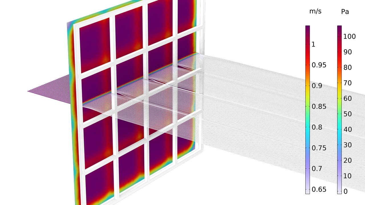
Many systems involve the combination of open and porous domains, such as filters and catalytic converters. For these systems, it is often beneficial to use RANS turbulence models in both the open and porous domains. In the Porous medium turbulence model list, there are now three formulation options: Nakayama-Kuwahara, Pedras-de Lemos, and Default (which combines the other two models). This feature is now available in the following interfaces:
- Turbulent Flow, k-ε
- Turbulent Flow, Realizable k-ε
- Turbulent Flow, Low Re k-ε
- Turbulent Flow, k-ω
- Turbulent Flow, SST
- Turbulent Flow, v2-f
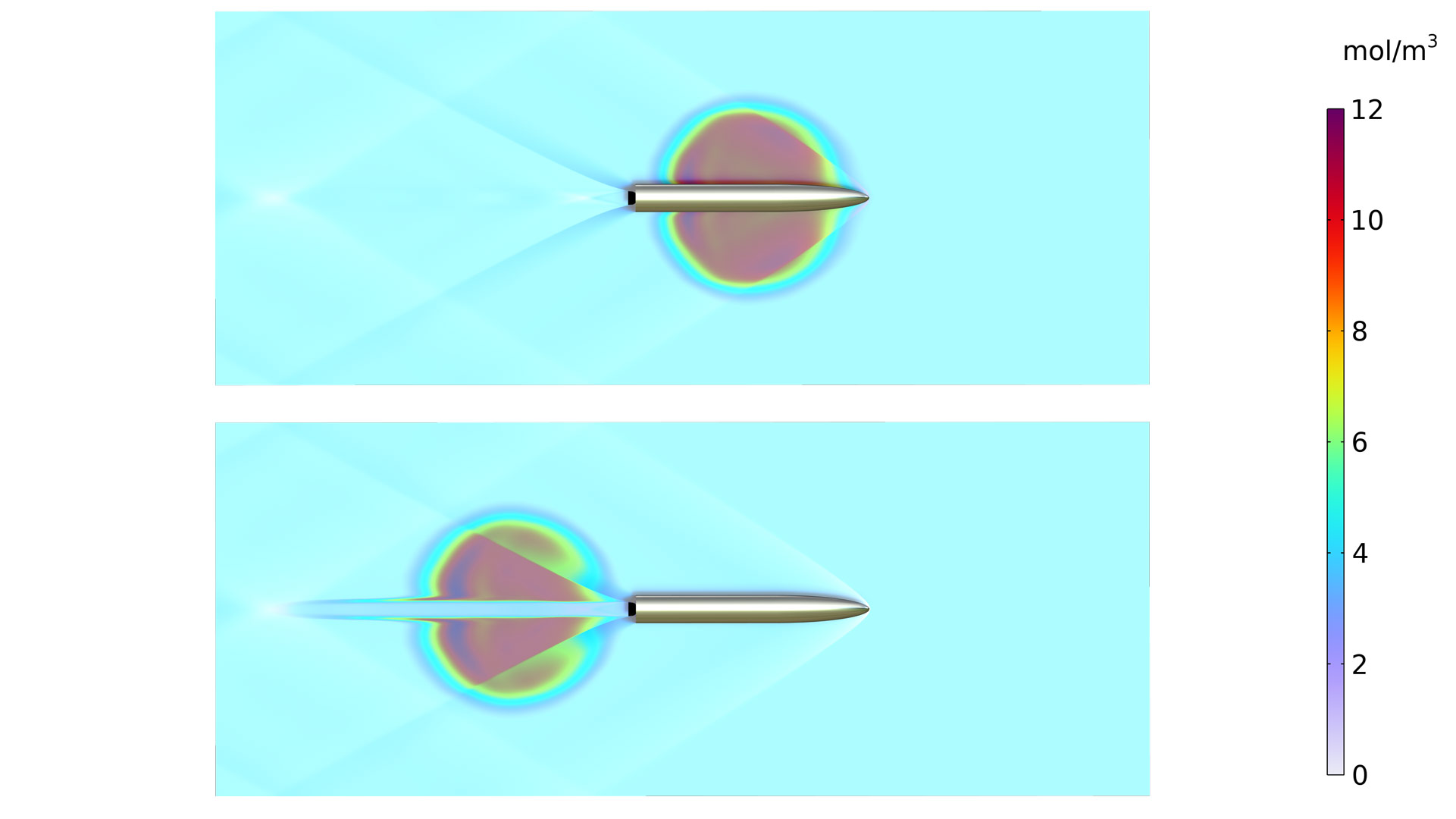
High Mach Number Reacting Flow Interfaces
The ability to model chemical species transport and reactions in combination with high Mach number flow is now available for both concentrated and diluted solutions. Under the Chemical Species Transport branch in the Model Wizard, the High Mach Number Reacting Flow interfaces contain two variants that combine fully compressible flow with the Transport of Diluted Species interface or the Transport of Concentrated Species interface (which requires a license to the Chemical Reaction Engineering Module). These interfaces are typically used for modeling gas-phase transport and reactions. In addition, with the new functionality you have the option to administrate complex chemical reaction mechanisms using the Chemistry feature that is available in the Chemical Reaction Engineering Module.
Multiphase Materials for Multiphase Flow Couplings
For the Two-Phase Flow, Level Set, Two-Phase Flow, Phase Field, and Three-Phase Flow, Phase Field multiphysics couplings, there is now the option to include effective material properties from a Multiphase Material node, with built-in mixing rules. This is especially efficient when coupling these multiphysics interfaces with other physics, such as heat transfer or electrostatics, since the multiphase material will use appropriate mixing rules for nonfluid material properties. In older versions, this would require you to write user-defined expressions based on the volume fraction of each fluid phase to compute the effective material properties used in each physics interface.
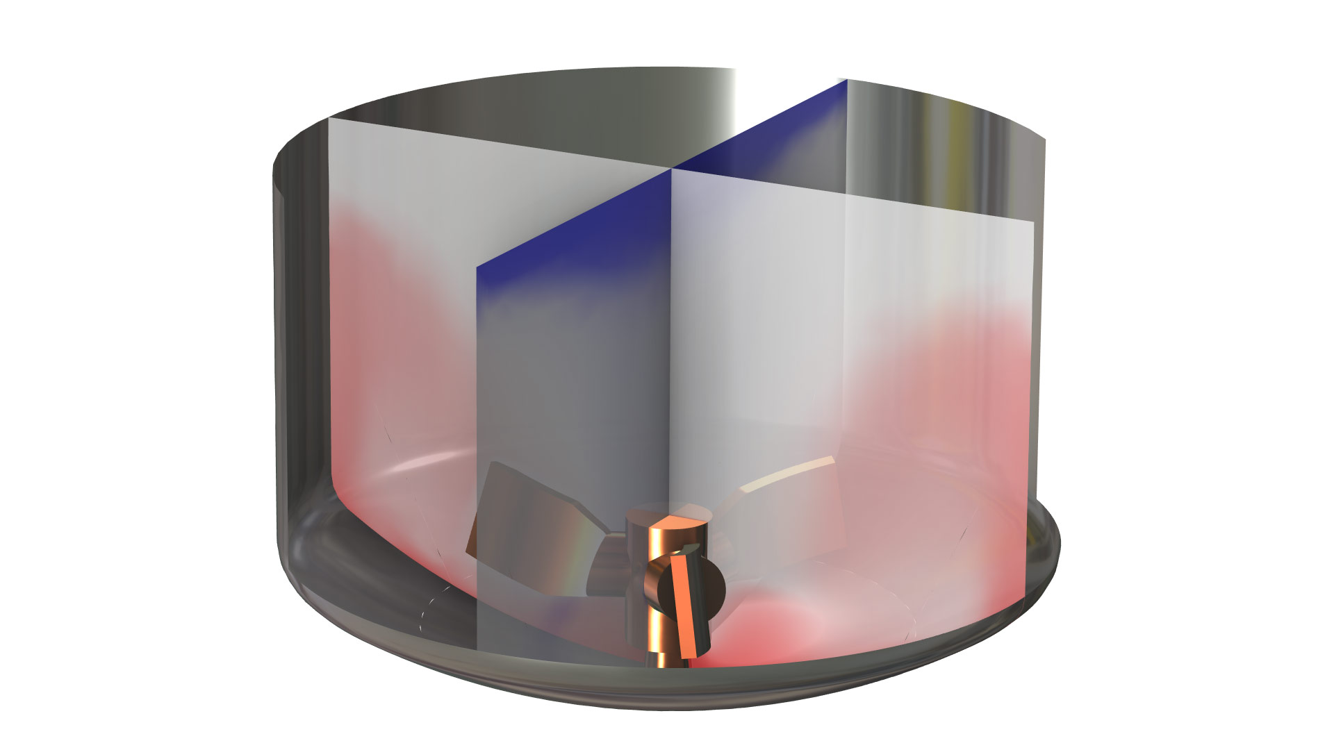
Liquid–air interface in a Taylor cone model. A liquid is displaced by the electrostatic forces caused by an electric field acting on the thin fluid–fluid interface. The relative permittivity used in the Electrostatics interfaces is computed by a multiphase material.
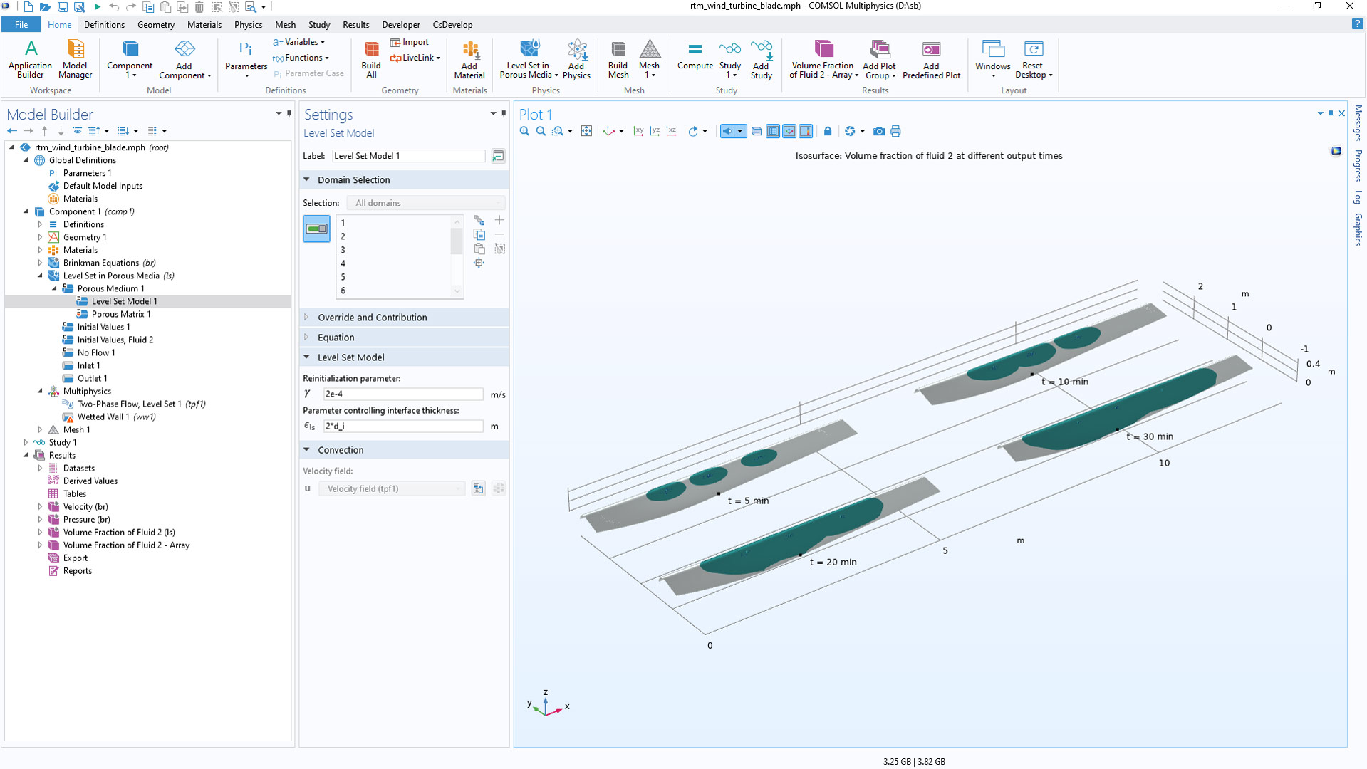
New Level Set in Porous Media Interface
The new Level Set in Porous Media interface includes a Porous Medium feature that can link to the definition of porosity given in the Porous Material node. This feature is also available in the Level Set interface and in the Brinkman Equations, Two-Phase Flow, Level Set multiphysics interface. View these features in the new Resin Transfer Molding of a Wind Turbine Blade tutorial model.
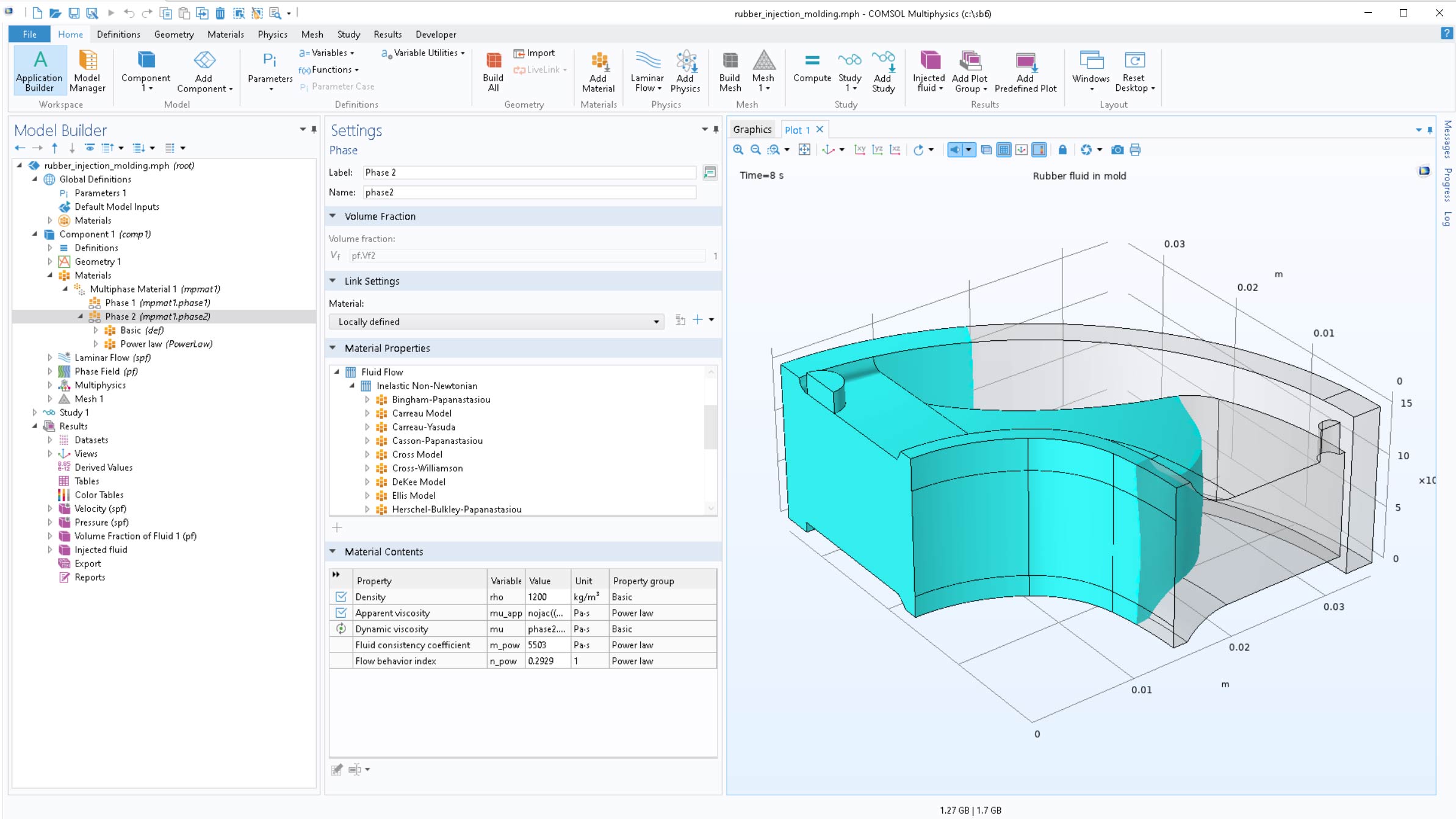
Inelastic Non-Newtonian Material Property Groups
Dedicated material property groups have been added for all available inelastic non-Newtonian models. Each material property group contains all necessary material parameters as well as the apparent viscosity expression. It picks up the shear rate from a Fluid Flow interface to define the dynamic viscosity for fluid by means of a synchronization rule. Thus, an inelastic non-Newtonian model can be selected directly by adding the corresponding Material Properties group as a subnode to a material node.
Improved Performance for CFD
The symmetrically coupled Gauss–Seidel (SCGS) method, used by many CFD applications, has been improved with better default settings. In many cases, this provides a 30% reduction in CPU time. Furthermore, the memory requirement for multigrid solvers with cluster computing has been reduced by up to 25%.
Dispersed Two-Phase Flow with Species Transport
The ability to model chemical species transport and reactions in two-phase flow is greatly enhanced by the new Dispersed Two-Phase Flow with Species Transport interface. This new multiphysics interface describes chemical species transport between two phases consisting of liquid droplets or gas bubbles in a continuous liquid phase. The functionality can be used to model separation processes, such as liquid–liquid extractions and wet scrubbing of process exhaust gases. Such two-phase systems are common in both the bulk and fine chemical industries.
Thin Barrier Multiphysics Coupling
The Multiphase Flow in Porous Media interface contains a new Thin Barrier multiphysics coupling. This feature is optional and makes it possible to add a thin layer that acts as resistance for flow fields of all phases, without having to mesh the layer's thickness.
Enhanced Thermal Wall Functions for Viscous Dissipation
In the Nonisothermal Flow coupling under its Heat Transfer Turbulence settings, a new Thermal wall function setting is available for RANS turbulence models. There are two options available: Standard, which is suitable for most configurations, and High viscous dissipation at wall, which accounts for viscous dissipation in the boundary layer. This is needed for accurate results in the case of fast internal flow, especially for narrow paths or if the fluid is very viscous.
New and Updated Tutorial Models
COMSOL Multiphysics® version 6.1 brings new and updated tutorial models to the CFD Module.
Resin Transfer Molding of a Wind Turbine Blade
Application Library Title:
rtm_wind_turbine_blade
Download from the Application Gallery
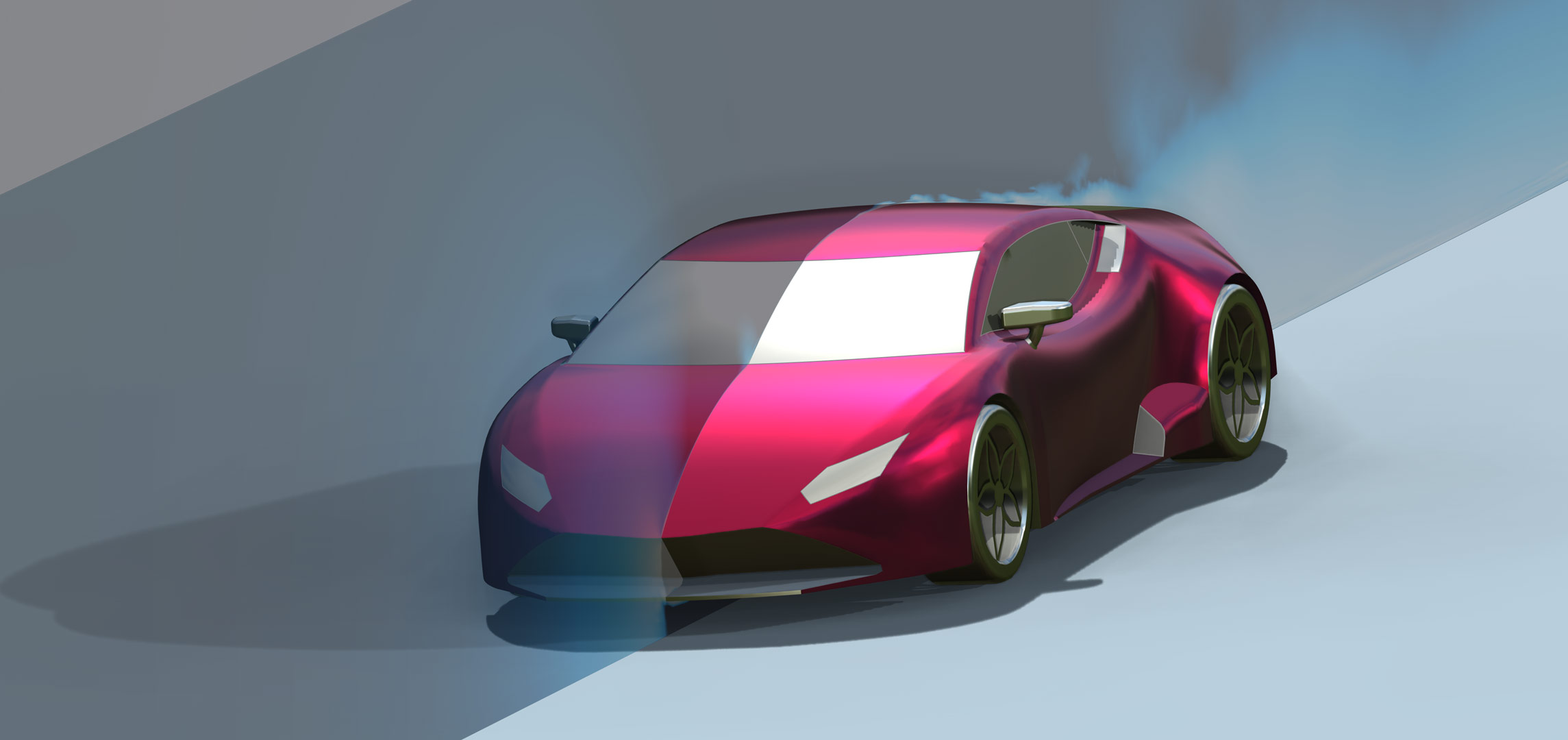
Fluid–Structure Interaction on a Sports Car Door
Application Library Title:
sports_car_fsi
Download from the Application Gallery
Transonic Flow over the ONERA M6 Wing
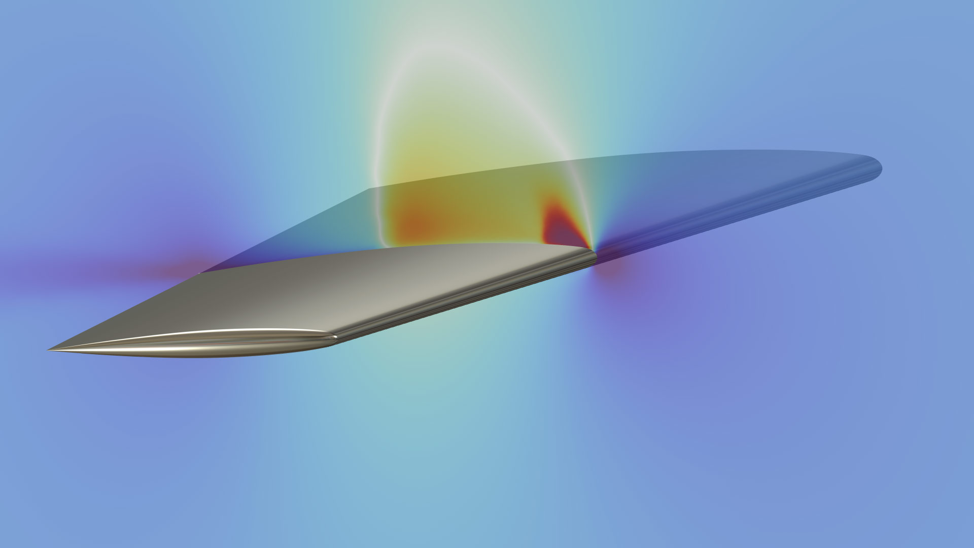
Application Library Title:
onera_m6_wing
Download from the Application Gallery
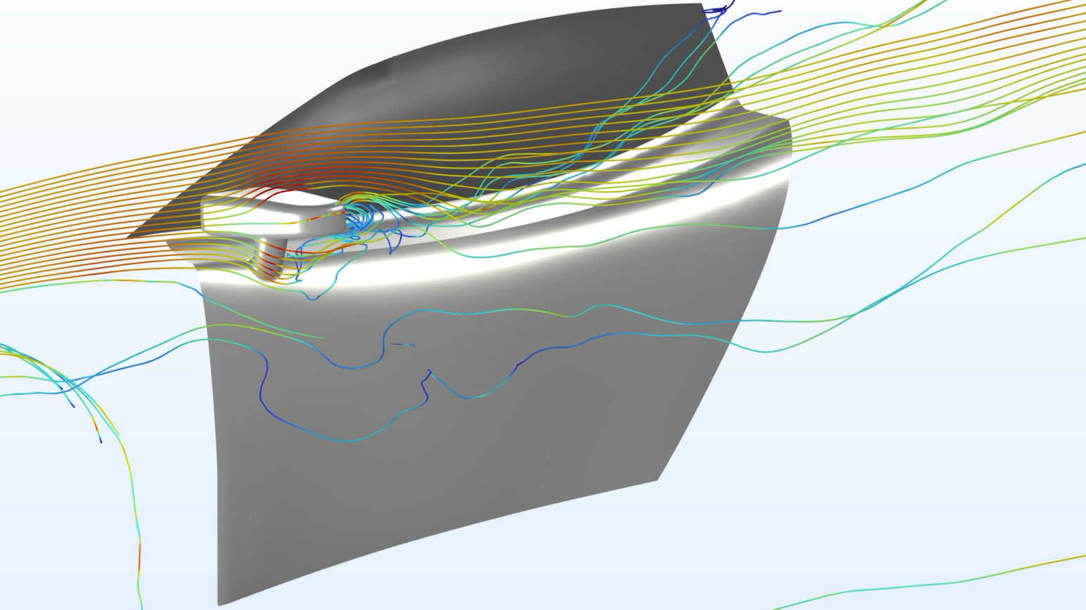
Large Eddy Simulation of a 3D Hill Geometry
Application Library Title:
les_3d_hill
Download from the Application Gallery
Three-Phase Mixer (requires the Mixer Module)
Application Library Title:
three_phase_mixer
Download from the Application Gallery