support@comsol.com
Acoustics Module Updates
For users of the Acoustics Module, COMSOL Multiphysics® version 6.1 provides functionality for simulating acoustic streaming, makes it possible to include the effects of fluid flow in convected acoustics using a time-explicit solver, and introduces lumped speaker boundary conditions for thermoviscous acoustics. Read about these updates and more below.
Simulation of Acoustic Streaming
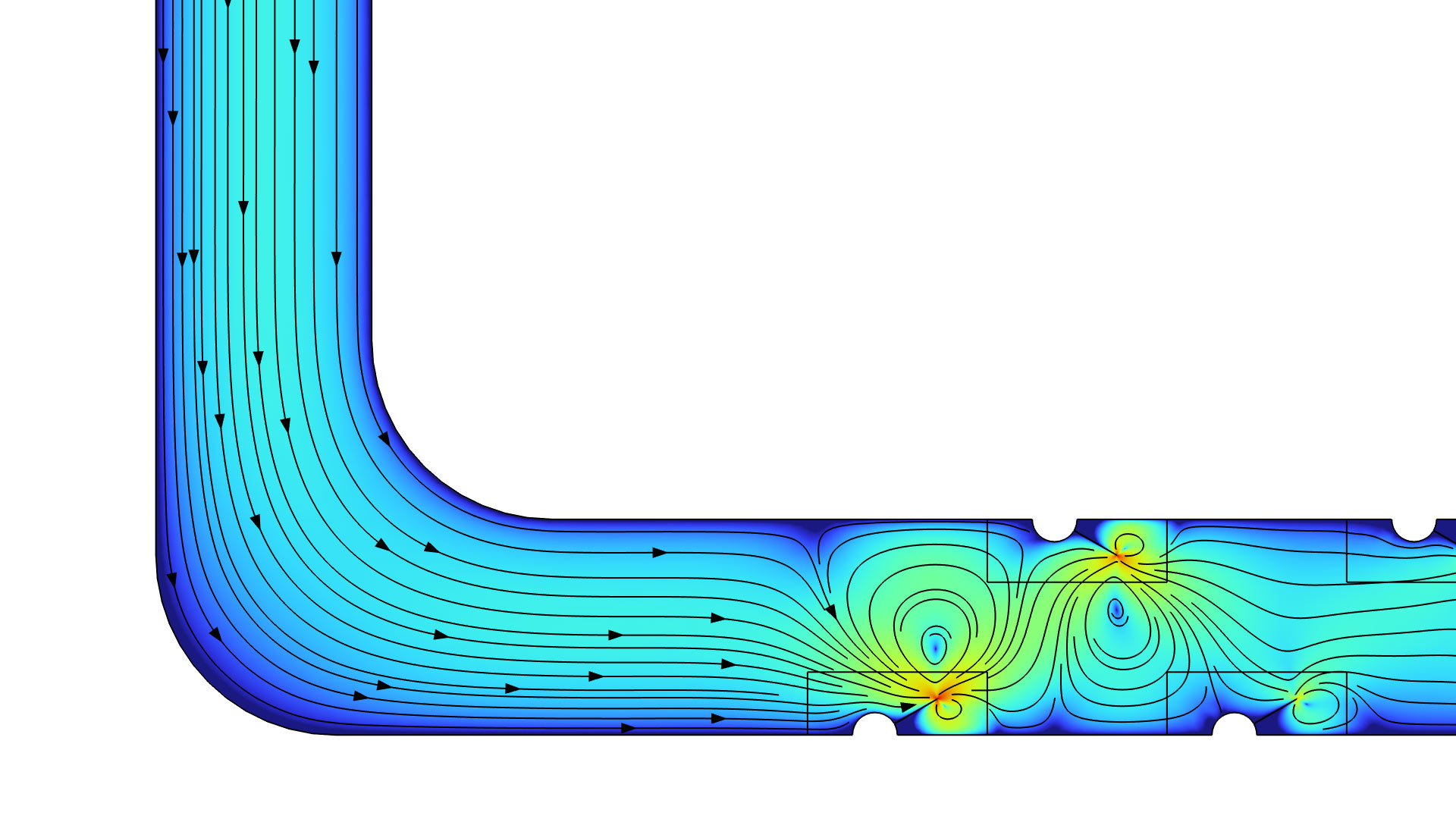
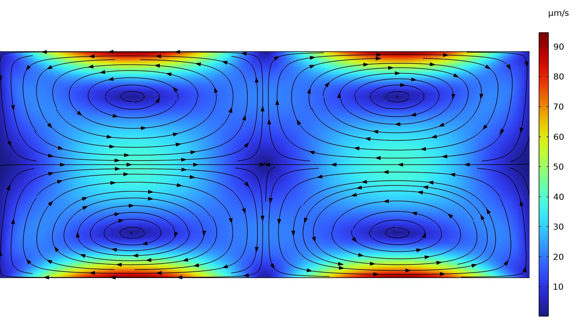
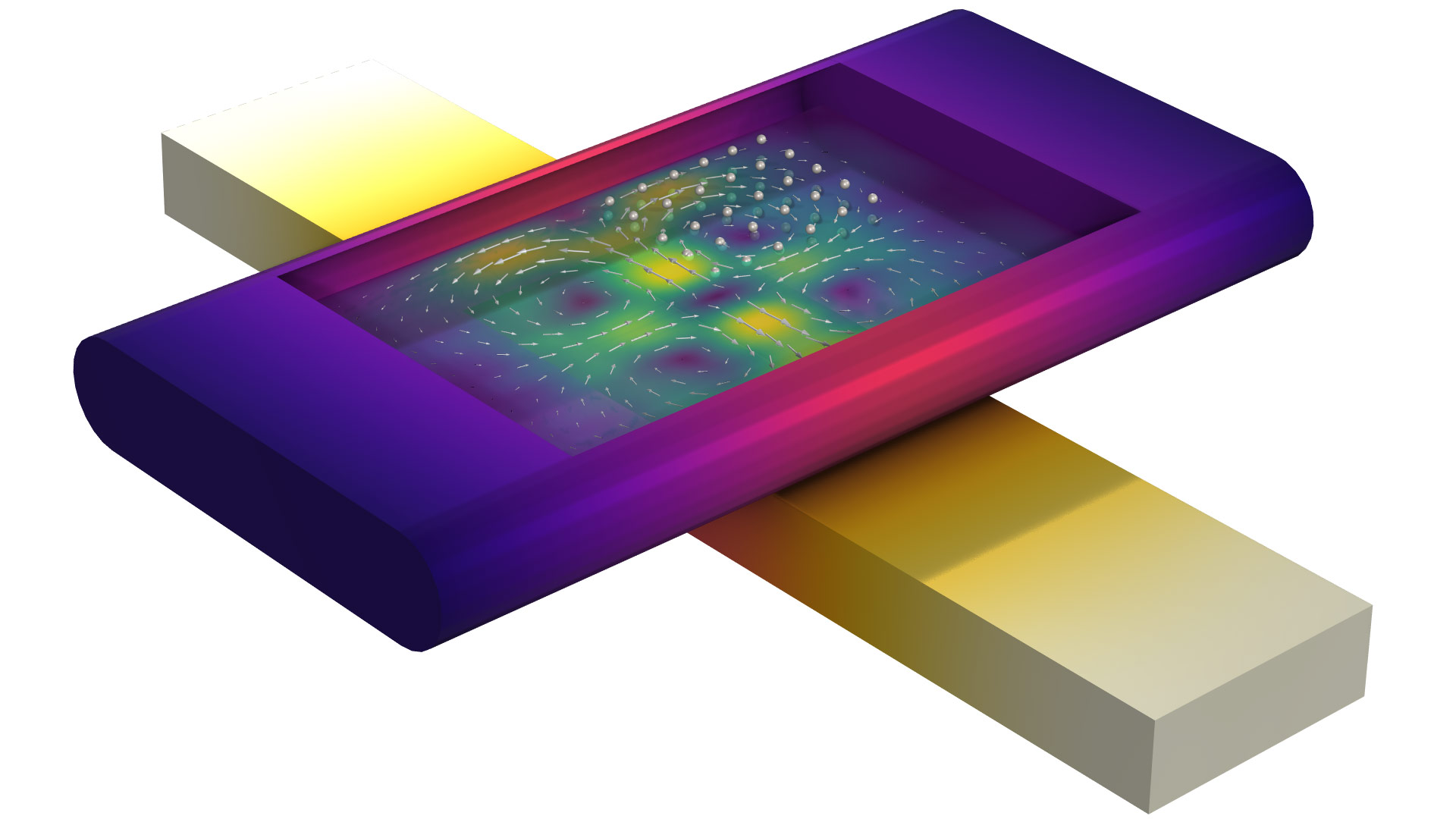
Acoustic streaming, that is, the fluid flow induced by an acoustic field, is important in microfluidics and lab-on-a-chip systems for applications such as particle handling, the mixing of fluids, and microfluidic pumps. The new acoustic streaming functionality in version 6.1 computes the forces, stresses, and boundary slip velocities that the acoustic field induces in a fluid in order to generate a flow field.
There are two new multiphysics interfaces for acoustic streaming simulations: Acoustic Streaming from Pressure Acoustics and Acoustic Streaming from Thermoviscous Acoustics. When you add either of these interfaces, two multiphysics couplings, the Acoustic Streaming Domain Coupling and Acoustic Streaming Boundary Coupling, are automatically created to couple a frequency-domain acoustic field with a stationary or time-dependent fluid flow. You can view these new multiphysics capabilities in the following tutorial models:
- Application Library Title: acoustic_microfluidic_pump
- Application Library Title: acoustic_streaming_microchannel_cross_section
- Download from the Application Gallery: 3D Acoustic Trap and Thermoacoustic Streaming in Glass Capillary
- Download from the Application Gallery: Opto-Acoustophoretic Effect in an Acoustofluidic Trap
Particles moving in an acoustic trap due to radiation forces and streaming in a glass capillary. Here, the small particles' movement is dominated by viscous drag forces.
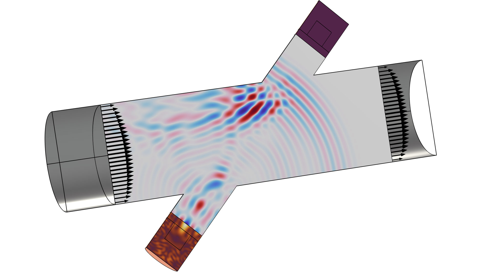
Stationary Background Flow for Convected Acoustic–Structure Interaction, Time-Explicit Simulations
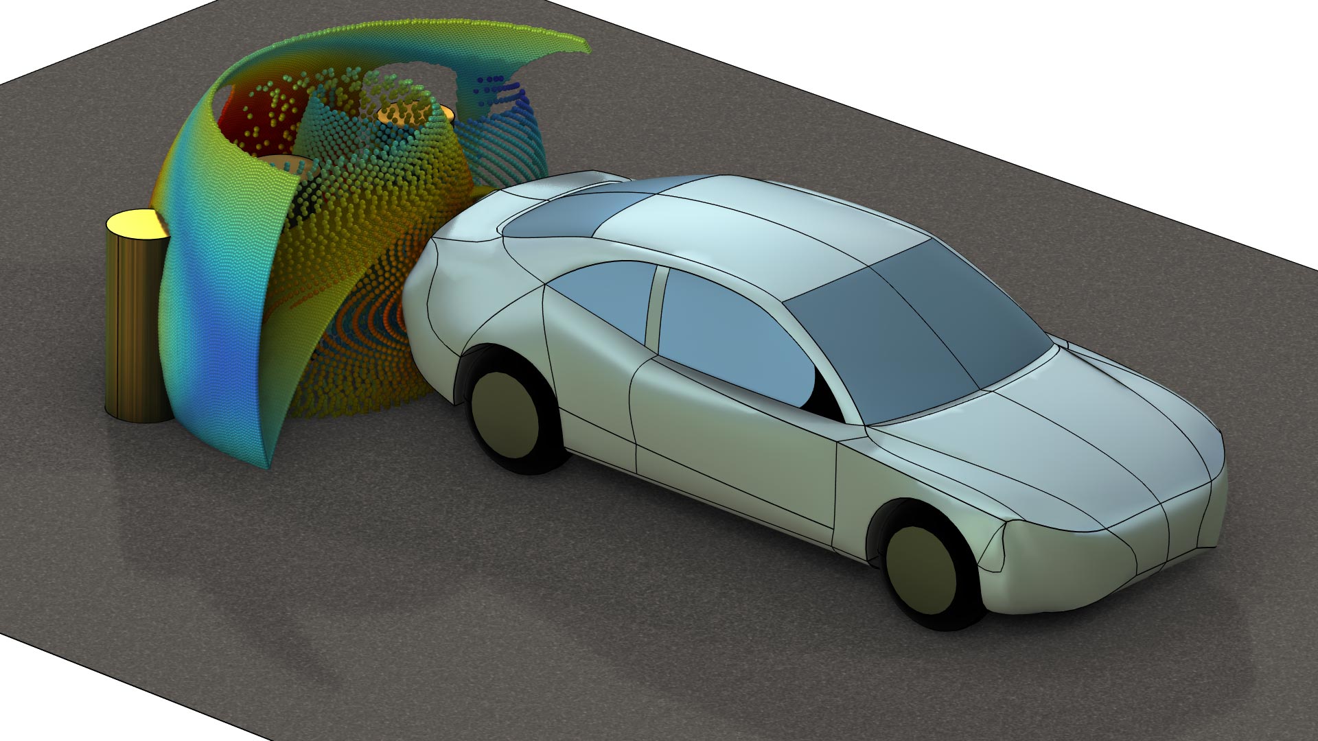
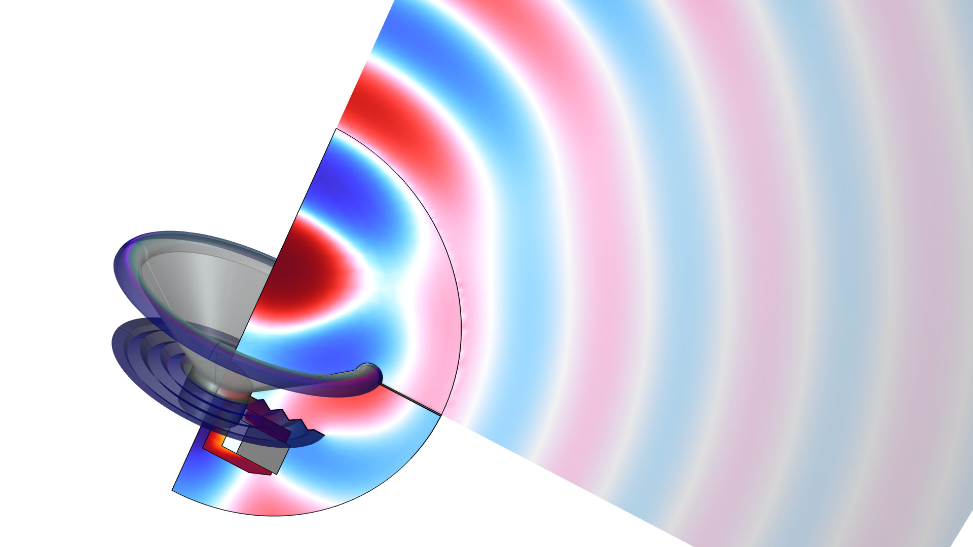
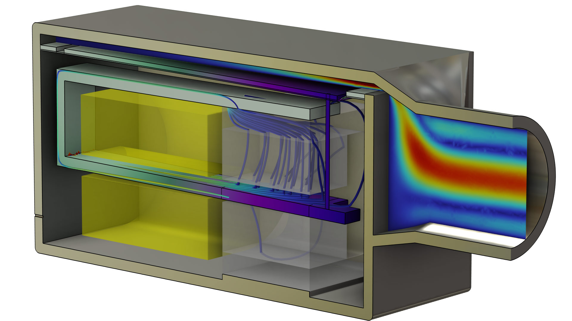
New functionality makes it possible to model convected acoustic–structure interaction (vibroacoustics in the presence of a stationary background flow) for large transient models, using the time-explicit formulation. There are two new multiphysics couplings for this purpose, Convected Acoustic-Structure Boundary, Time Explicit and Pair Convected Acoustic-Structure Boundary, Time Explicit, which are used to couple the Convected Wave Equation, Time Explicit interface with the Elastic Waves, Time Explicit interface. The conditions are added on the boundary (or pair selection) between the fluid domain and the solid domain. A common application is for modeling flowmeter systems, as seen in the Ultrasonic Flowmeter with Piezoelectric Transducers model.
Propagation of the acoustic signal on the symmetry plane in an ultrasonic flowmeter. The model includes a fully coupled physical setup with piezoelectric transducers, matching backing layers, and a background flow.
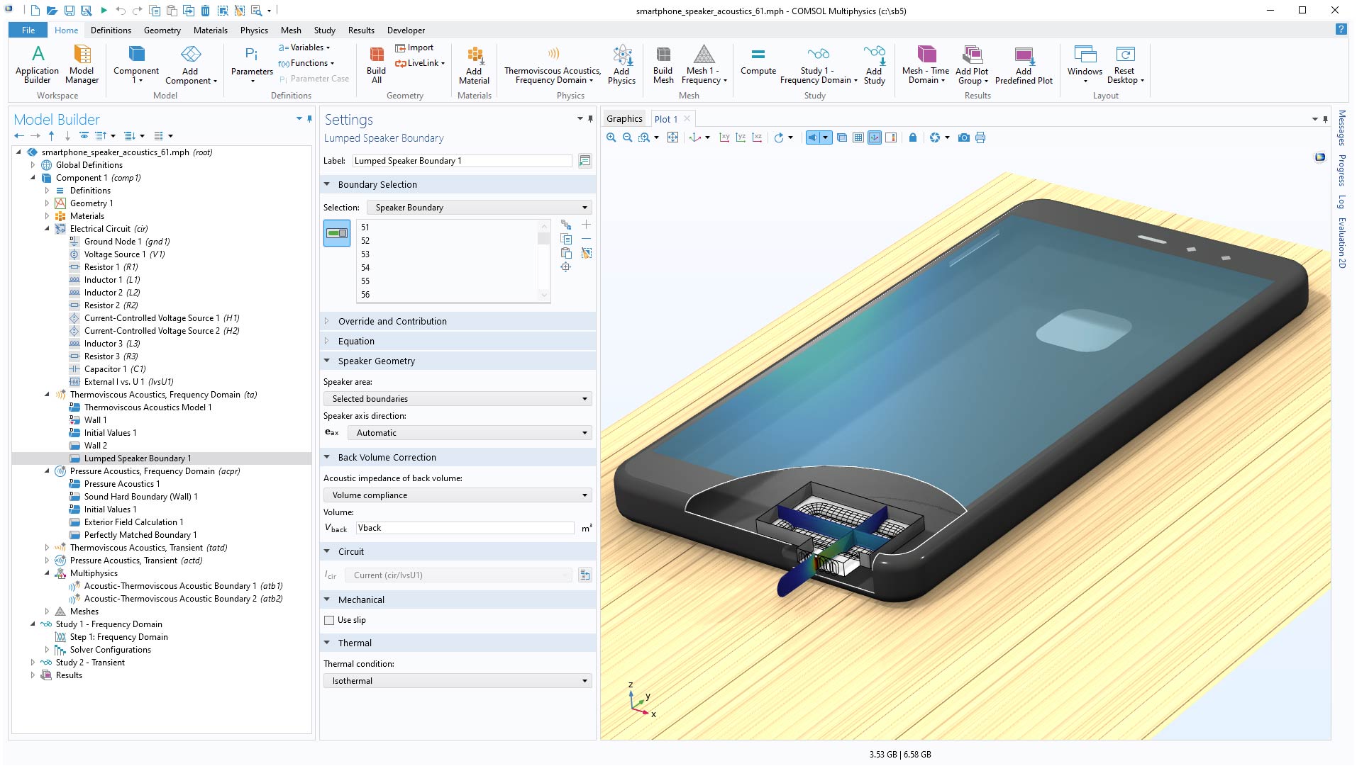
Lumped Speaker Boundary for Thermoviscous Acoustics
The Lumped Speaker Boundary and Interior Lumped Speaker Boundary features are now available for thermoviscous acoustics in the frequency and time domains. This completes and extends the existing boundary conditions in the Pressure Acoustics interfaces. With these boundary conditions, it is easier to set up and model microspeakers with hybrid lumped-finite element method (FEM) representations in thermoviscous acoustics. The lumped representations are often accurate over a larger frequency range for microtransducers, as breakup effects occur outside the intended frequency range. In the time domain, nonlinear effects can be included through large signal parameters like CMS(x), BL(x), or RMS(v).
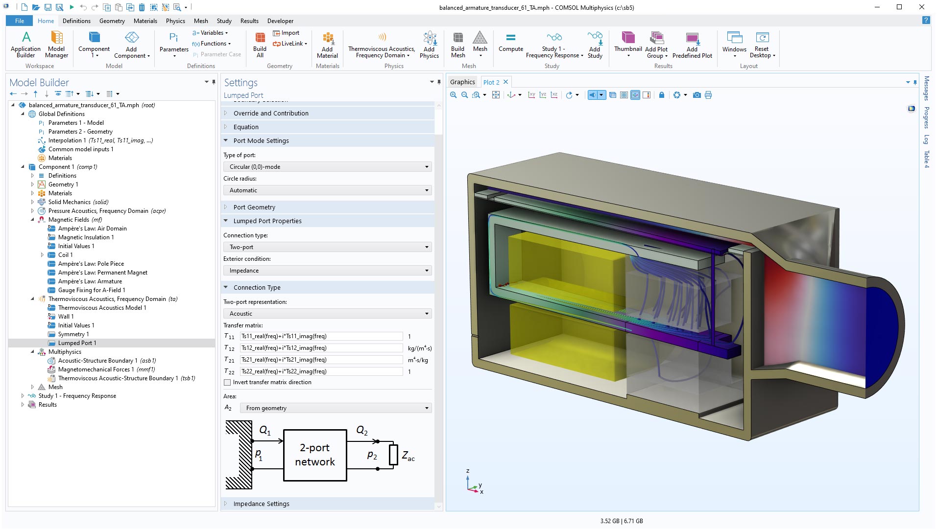
Lumped Port in Thermoviscous Acoustics
The Lumped Port feature has been added to the Thermoviscous Acoustics, Frequency Domain interface. This feature connects a waveguide or duct inlet or outlet to a lumped representation element; this can be an Electrical Circuit interface (a lumped electroacoustic representation), a two-port network defined through a transfer matrix, or a lumped representation of a waveguide. In summary, it couples the end of a waveguide with an exterior system that has a given acoustic lumped representation. When using the lumped port representation, it is assumed that only plane pressure waves (the (0,0)-mode) propagate in the acoustic waveguide. The condition ensures a mathematically and physically consistent coupling that includes the thermoviscous boundary layers in the waveguide.
Thermoviscous–Thermoelasticity Multiphysics Coupling
New functionality makes it possible to accurately model the vibrating response of MEMS devices by including a more detailed description of damping. There are two new multiphysics interfaces for modeling thermoviscous acoustics coupled with thermoelasticity (one each for the frequency and time domains): the Thermoviscous Acoustic-Thermoelasticity Interaction, Frequency Domain interface and the Thermoviscous Acoustic-Thermoelasticity Interaction, Transient interface. When adding either of the interfaces, the Thermoviscous Acoustics, Solid Mechanics, and Heat Transfer in Solids interfaces are included in the model, as well as a Thermoelasticity multiphysics coupling and the new Thermoviscous Acoustic-Thermoelasticity Boundary multiphysics coupling. The new multiphysics interfaces couple the displacement and temperature field in the solid domain with the acoustic variations in the pressure, velocity, and temperature in the fluid domain. The formulation relies on a perturbation approach for all of the fields. You can view the new multiphysics capabilities in the Prestressed Micromirror Vibrations: Thermoviscous-Thermoelasticity Coupling tutorial model.
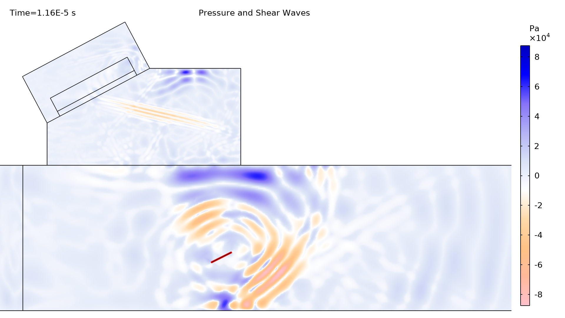
Fracture Boundary Condition for Elastic Waves
The new Fracture boundary condition, available in the Elastic Waves, Time Explicit physics interface, is used to treat two elastic domains with imperfect bonding. The fracture can be a thin elastic layer, fluid-filled layer, or discontinuity in elastic materials (an interior boundary). Several options exist for specifying the properties of the thin elastic domain. Typical applications are for modeling nondestructive testing (NDT) applications, such as inspecting the response of delamination regions or other defects, or for modeling wave propagation in fractured solid media in the oil and gas industry. You can see this feature in the Angle Beam Nondestructive Testing model.

Performance Improvements for Time-Explicit Interfaces
Several important solver performance improvements, as well as improved formulations on the physics side, apply to all of the time-explicit acoustics interfaces. When running simulations using the time-explicit acoustics interfaces, which are based on the discontinuous Galerkin (dG) method, COMSOL Multiphysics® now supports solving for more than 2 billion degrees of freedom (DOFs).
Piezoelectric Waves, Time Explicit Interface
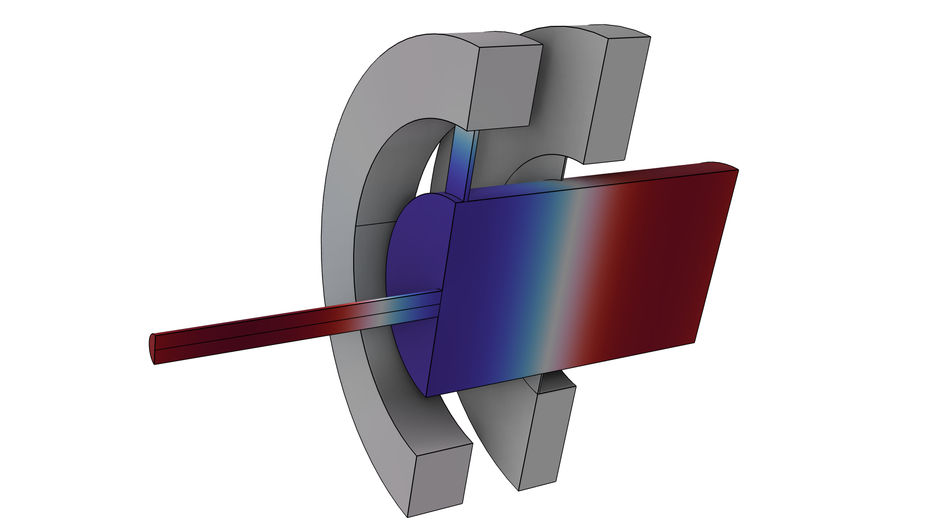
When running models involving piezoelectric effects using a time-explicit method, there is a new time-stepping strategy for the electrostatic part of the problem that improves performance. The performance when solving large piezoelectric time-explicit models on a cluster architecture has also been improved. The piezoelectric multiphysics relies on a mixed dG-algebraic FEM formulation, which now has the same performance as a pure dG time-explicit problem. As an example, the Ultrasonic Flowmeter with Piezoelectric Transducers model (now with a finer mesh, resolving double the frequency) runs on eight nodes on a cluster architecture and exhibits a speedup of 35%. Furthermore, the model solves for 75,600,000 DOFs, with 3700 algebraic-FEM DOFs (the voltage in the piezoelectric domains).
Pressure Acoustics, Time Explicit Interface
The Impedance boundary conditions now use an improved numerical flux formulation for stability, ensuring that both acoustically hard and soft boundaries result in a stable solution. Additionally, two new conditions have been added for modeling a transfer impedance setup: Interior Impedance and Pair Impedance. Both conditions also take advantage of the improved numerical flux from the impedance condition.
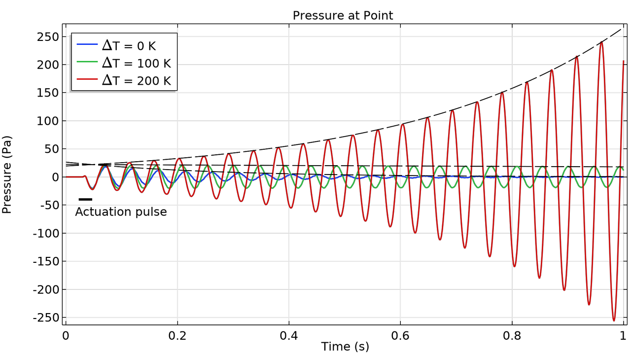
There is also improved performance when solving systems of ordinary differential equations (ODEs) together with the Pressure Acoustics, Time Explicit interface. This is useful when modeling frequency-dependent impedance conditions in the time domain. You can see an example of this in the Full-Wave Time-Domain Room Acoustics with Frequency-Dependent Impedance tutorial model.
Propagation of a Gaussian pulse with a 7 kHz carrier signal inside a room. The model solves for 2.2x10⁹ degrees of freedom (DOFs) and includes ODEs for modeling a frequency-dependent absorbing ceiling.
Elastic Waves, Time Explicit Interface
In 2D and 2D axisymmetric models, the underlying equations have been reformulated to be more efficient for these specific cases. In 2D models, there is a new option to include or exclude the computation of the out-of-plane components. When included, the representation is the so-called 2.5D formulation; otherwise, it is the plane-strain formulation. In 2D axisymmetric models, the out-of-plane components are always excluded. As an example, the number of DOFs solved for in the Propagation of Seismic Waves Through Earth model has been reduced from 17.2x10⁶ to 12.2x10⁶. On the same workstation, the computation time for this model has been decreased from 15 hr and 40 min to 12 hr and 20 min.
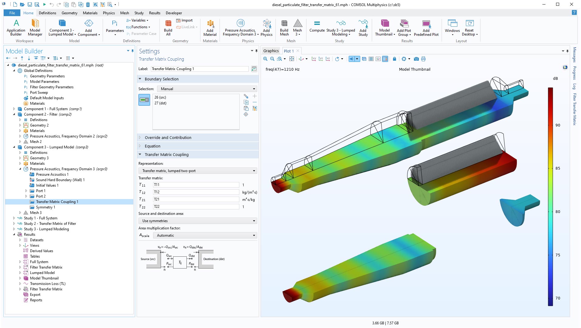
New Transfer Matrix Coupling Boundary Condition in Pressure Acoustics, Frequency Domain
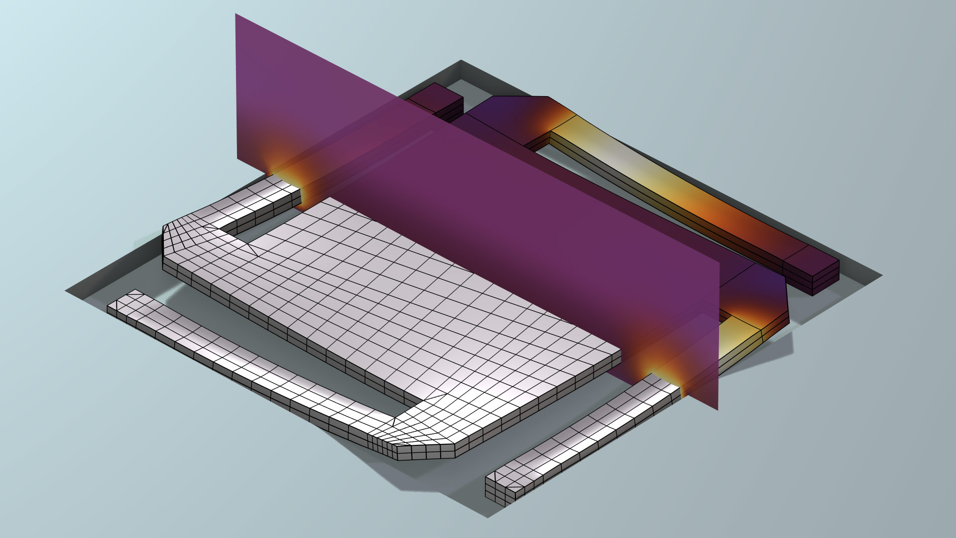
The new Transfer Matrix Coupling boundary feature in the Pressure Acoustics, Frequency Domain interface is used to couple two boundaries (source and destination) using a transfer matrix representation. The transfer matrix is a reduced or lumped representation of the physical domain connecting the two boundaries. The feature has two options, a so-called pointwise coupling and a lumped representation, and can be seen in the Diesel Particulate Filter Analysis Using an Acoustic Transfer Matrix model.
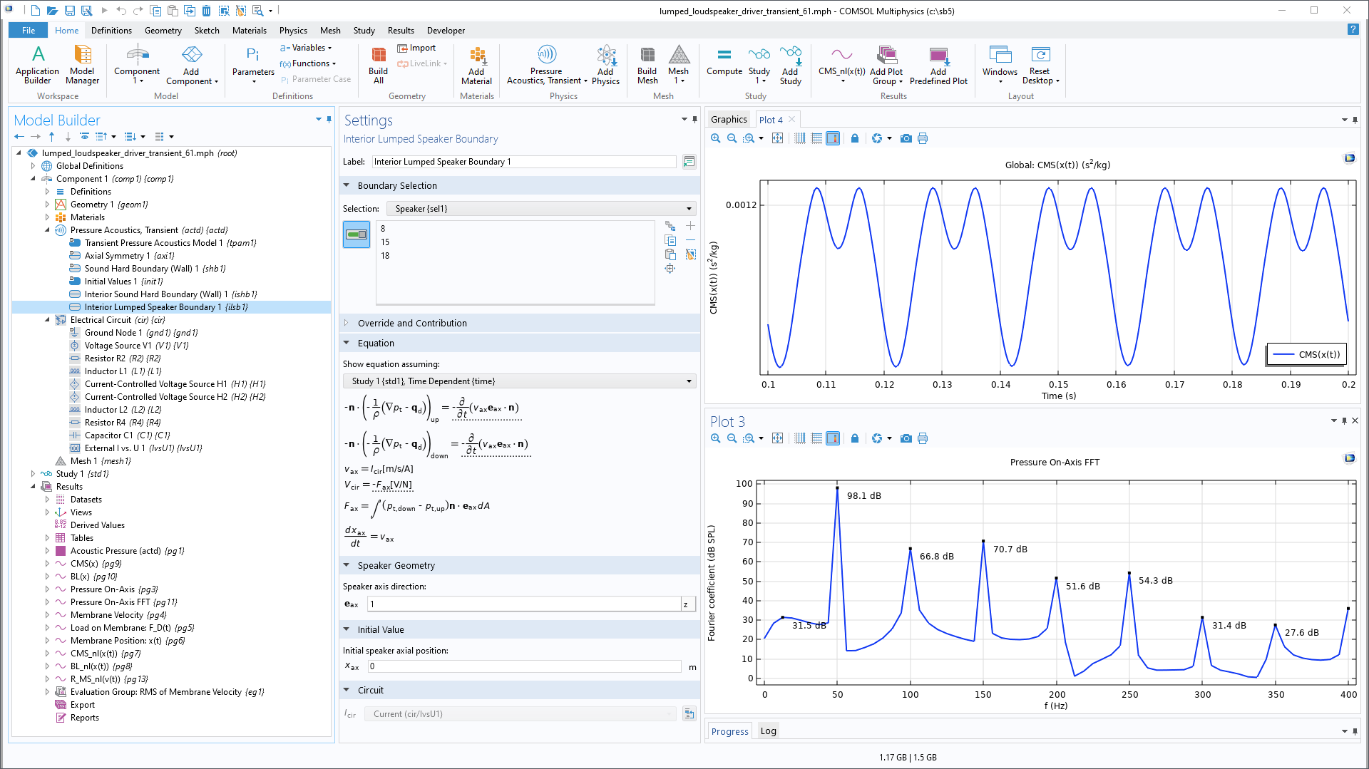
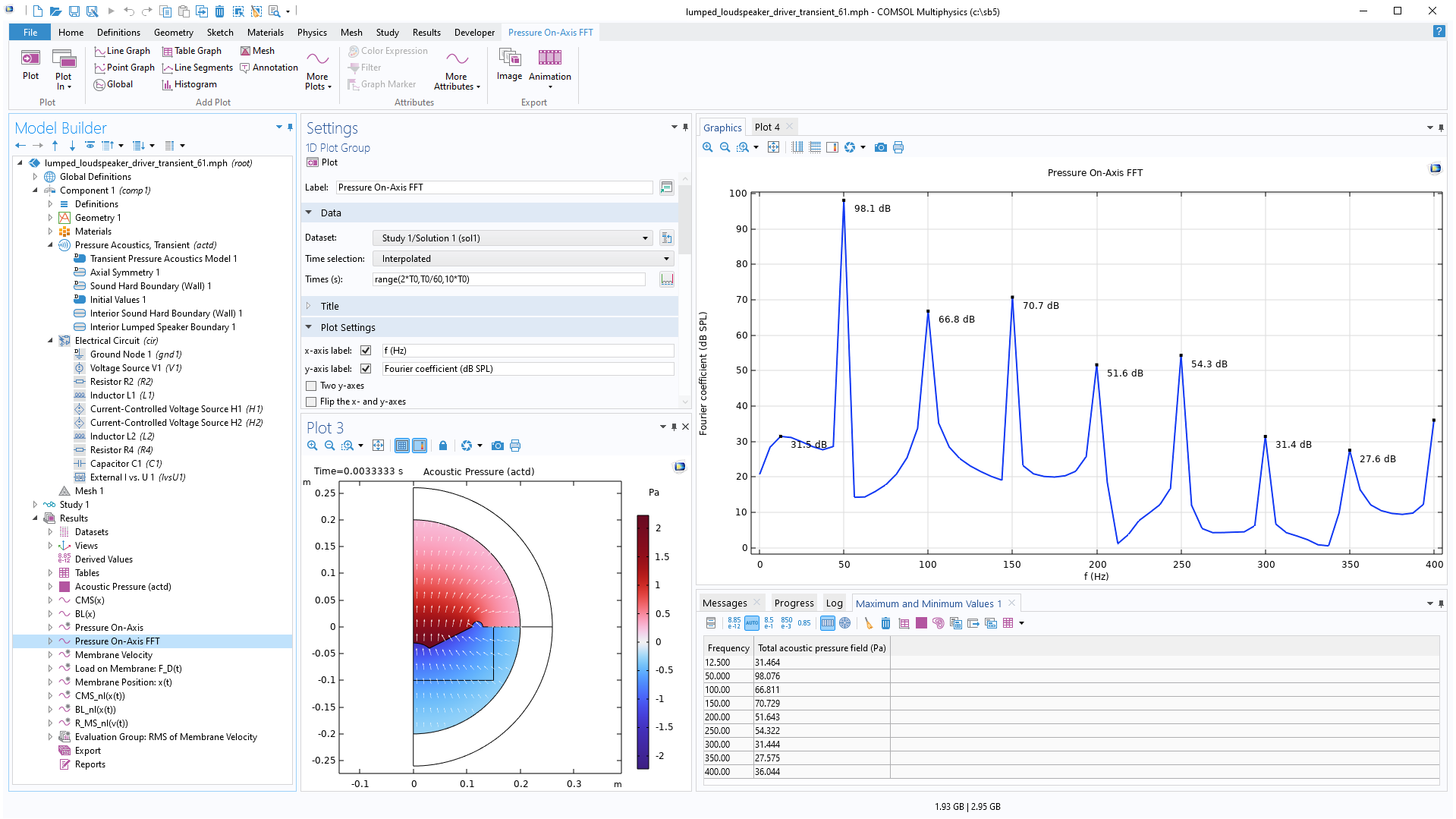
Lumped Speaker Boundary and Interior Lumped Speaker Boundary for Pressure Acoustics, Transient
The Lumped Speaker Boundary and Interior Lumped Speaker Boundary conditions have been added to the Pressure Acoustics, Transient interface to model hybrid lumped and FEM loudspeaker setups. This complements the features that already exist in the Pressure Acoustics, Frequency Domain interface. The condition sets up couplings between the boundary condition and an Electrical Circuit interface in order to set up models that can include large-signal parameters like CMS(x), BL(x), or RMS(v) in a simplified way. Predefined global variables exist for the axial position and velocity. You can see this functionality in the Lumped Loudspeaker Driver Transient Analysis with Nonlinear Large-Signal Parameters model.
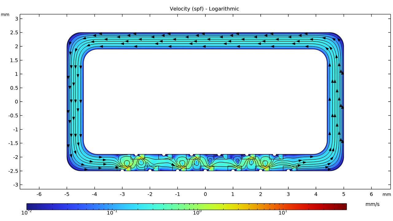
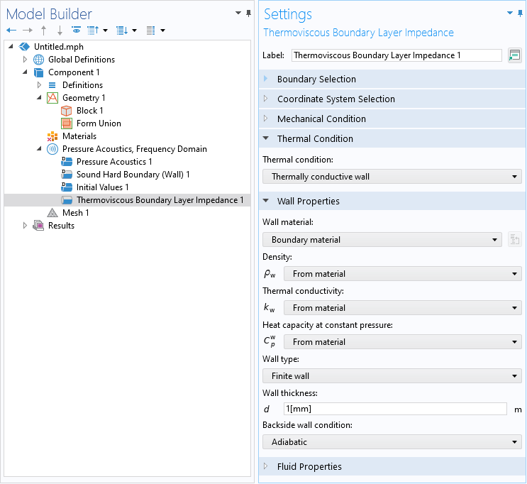
Extended Thermal Conditions in the Thermoviscous Boundary Layer Impedance Feature
A new Thermally conductive wall option has been added to the Thermoviscous Boundary Layer Impedance feature. This new option enables the modeling of nonideal thermal wall conditions using different analytical representations of walls of finite or infinite thickness. There are also new variables for the evaluation of the combined dissipated and transported energy (including convective terms) in the boundary layers. These variables are useful not only when modeling dissipation but also heating.
Porous Layer Impedance Options for Pressure Acoustics
The Porous layer option in the Impedance boundary condition has been updated with options for handling the impedance's dependency on the angle of incidence. The angle of incidence can be normal to the surface or set to a specific angle or direction. An Automatic option assigns an effective angle of incidence that is useful for room acoustics simulations with diffuse acoustic fields.
Physics-Controlled Mesh for Acoustics Physics
Physics-controlled mesh generation has been extended to more Acoustics interfaces. A physics-controlled mesh results in the generation of a good initial mesh that fulfills best meshing practices, such as resolving the wave phenomena and boundary layers. Physics-controlled mesh has been added for the following interfaces:
- Pressure Acoustics, Boundary Element
- Pressure Acoustics, Kirchhoff-Helmholtz
- Pressure Acoustics, Asymptotic Scattering
- Pressure Acoustics, Time Explicit
- Nonlinear Pressure Acoustics, Time Explicit
- Elastic Waves, Time Explicit
- Thermoviscous Acoustics, Frequency Domain
- Thermoviscous Acoustics, Transient
Speedup of Evaluations Based on the Kirchhoff–Helmholtz Kernel
Features that rely on the evaluation of the Kirchhoff–Helmholtz integral are now up to 50% faster than in version 6.0; the amount of speedup depends on the hardware and the complexity of the plot (most gain achieved for increasing complexity). One feature that benefits from these improvements is the Exterior Field Calculation feature, which is used in pressure acoustics for plotting the exterior field in results.
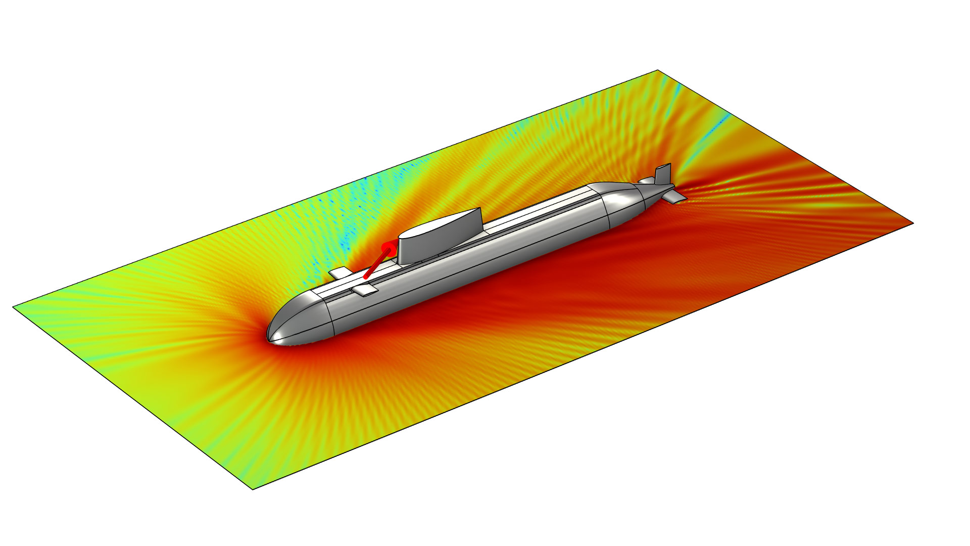
The actual computation time lies in the evaluation of the Kirchhoff–Helmholtz integral kernel. Therefore, these improvements (as well as how they affect the Exterior Field Calculation feature) are particularly important when using the high-frequency acoustics interfaces Pressure Acoustics, Asymptotic Scattering and Pressure Acoustics, Kirchhoff-Helmholtz. As an example, the evaluation time of the final plot, Scattered SPL, in the Submarine High-Frequency Asymptotic Scattering tutorial model has decreased by 25%.
Ray Acoustics Improvements
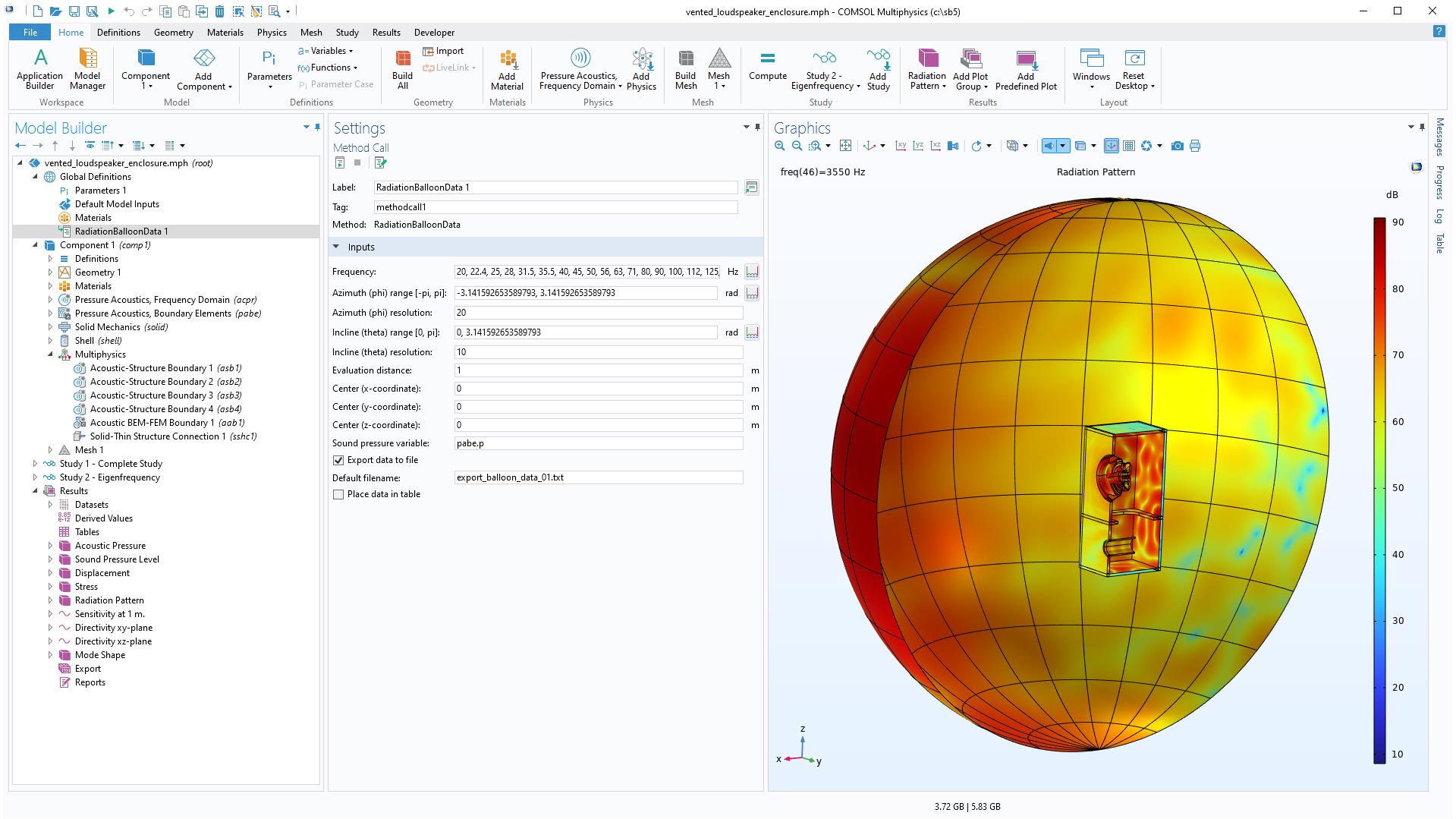
Export of Balloon Data with Method Call
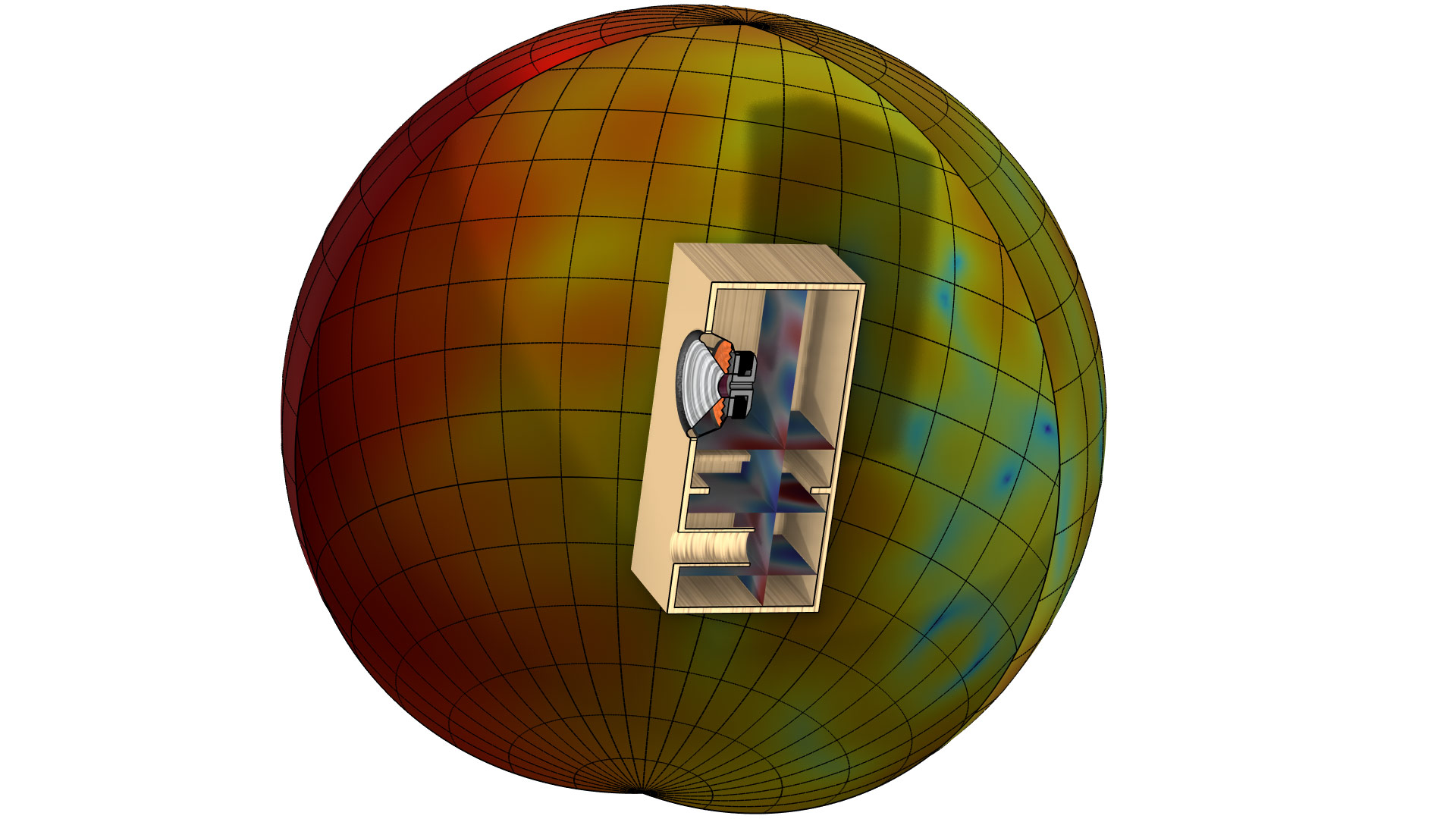
The Loudspeaker Driver in a Vented Enclosure model now includes a Method and Method Call that enable the export of loudspeaker radiation data (balloon plot) in a format suited for future use. This is an example of how custom export can be done with a method using the tools available in the Application Builder. The exported balloon data is also used to define a Source with Directivity feature in the Small Concert Hall Acoustics tutorial model.
Improved Pseudorandom Number Generation
The Ray Acoustics interface includes several features that rely on pseudorandom number generation (PRNG), such as conditional ray–boundary interaction and diffuse or isotropic scattering at boundaries. For such features, the calls to pseudorandom number generators have been extensively reviewed and revised. The new expressions are much less likely to incur correlations between random numbers that should be uncorrelated. This includes unwanted correlations between random boundary conditions acting on different rays as well as between randomly generated vector components.
Option to Only Store Accumulated Variables in Solution
Depending on your application, the accumulated variables, such as sound pressure level on boundaries, might be of more value than the position and direction of individual rays. To reduce file size, you now have the option to only retain the accumulated variables in the solution, discarding the degrees of freedom associated with the rays.
Release From Exterior Field
The Release From Exterior Field feature can now pick up exterior fields from the Pressure Acoustics, Kirchhoff-Helmholtz and Pressure Acoustics, Asymptotic Scattering interfaces. Moreover, the feature now handles solving for several frequencies in a parametric sweep.
Flow-Induced Noise Improvements
The Aeroacoustic Flow Source Coupling multiphysics feature now allows the flow source to be taken from the new Detached Eddy Simulation fluid flow interfaces. The Large Eddy Simulation fluid flow interface has several new features, including a synthetic turbulence option for inlets. For further details see the CFD Module Updates. The excess pressure terms are also now included in the Lighthill stress tensor; these describe, for example, the deviations from linear isentropic behavior if strong nonlinear effects occur in the source region or if a heat source is present in the flow simulation.
Solid Mechanics Interface in 1D
The Solid Mechanics interface is now available for 1D and 1D axisymmetric components and requires no additional product for the basic functionality. In the transverse directions, different combinations of plane stress, plane strain, and generalized plane strain can be selected. There are several multiphysics applications in, for example, battery modeling, acoustics, and thermal–structure interaction where a 1D model can be useful for providing important insights into a physical phenomenon. Note that functionality for intercalation strains in batteries is included in the Battery Design Module. For more advanced modeling, additional features are available with the Structural Mechanics Module, MEMS Module, Multibody Dynamics Module, or Acoustics Module.
New Method for Connecting Assemblies
Nitsche's method has been added to enforce continuity between boundaries in assemblies. It has two important advantages when compared with classical pointwise constraints:
- It causes significantly less local disturbances in the solution when the meshes on the two sides are not conforming.
- No constraints are added. As a result, there is no need to eliminate constraints, which is numerically sensitive and sometimes computationally heavy.
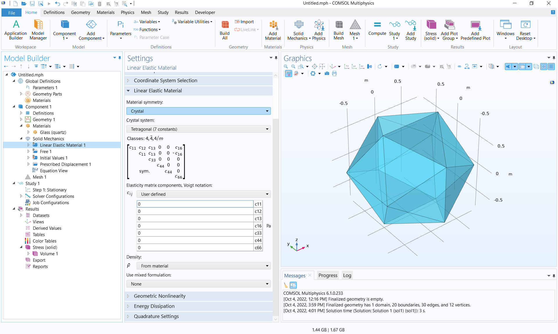
New Inputs for Anisotropic Materials
For the Linear Elastic Material feature, several new options for entering elastic constants have been added:
- Orthotropic materials can now be described by crystal data for seven different types of crystal systems: cubic, hexagonal, trigonal with six constants, trigonal with seven constants, tetragonal with six constants, tetragonal with seven constants, and orthorhombic.
- Input for transversely isotropic materials is supported, reducing the number of inputs for this class of materials.
- A general anisotropic material can now, in addition to the elasticity matrix, be represented by its compliance matrix.
Results in Local Coordinate Systems
It is now easy to define any arbitrary number of local coordinate systems by adding Local System Results nodes for the evaluation of common quantities in the Structural Mechanics interfaces. Among the available transformed quantities, you will find stresses, strains, displacements, and material properties.
Predefined Plot Suggestions
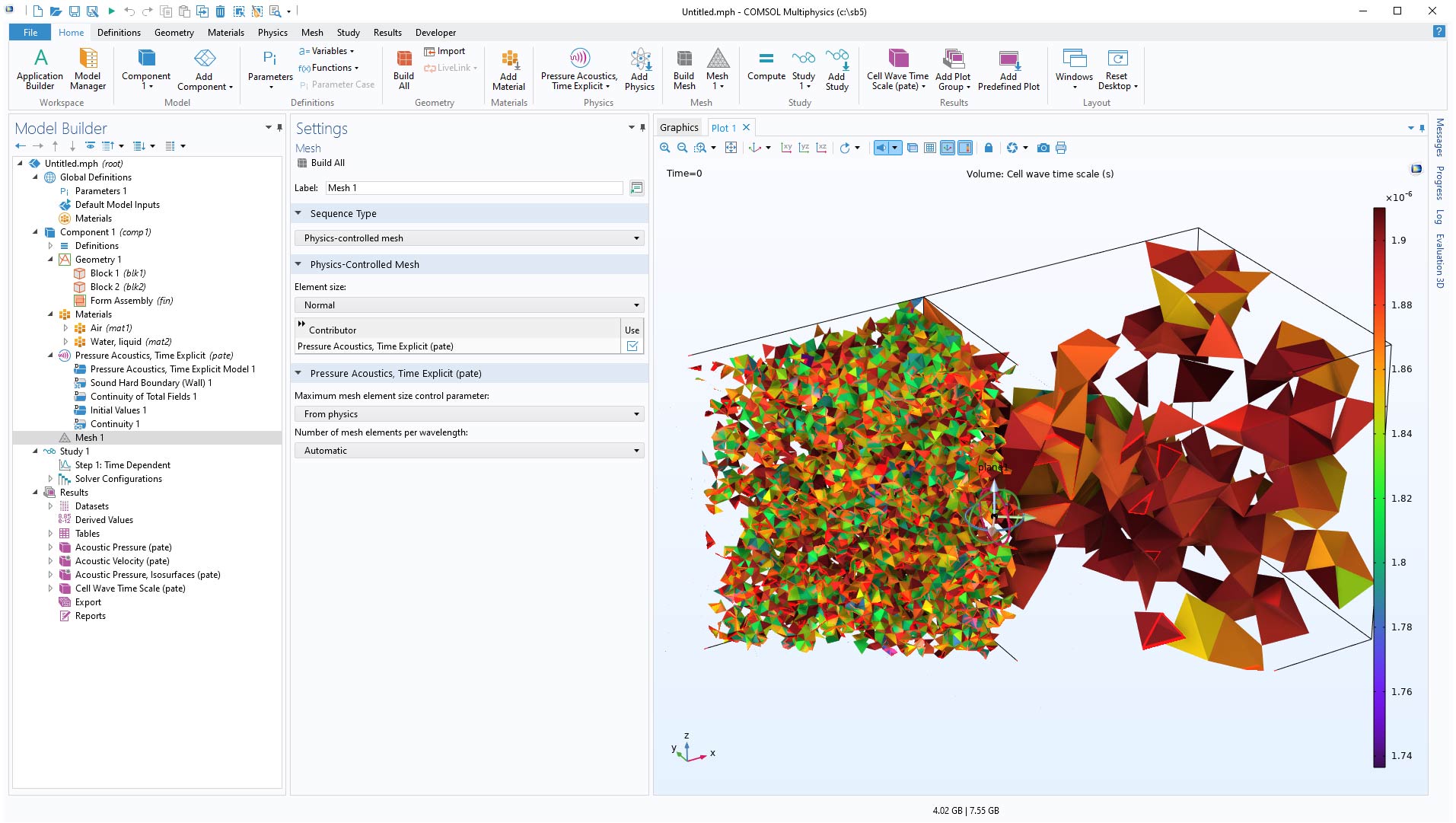
Several predefined acoustics plots have been added to the Add Predefined Plot menu in the Results tab of the ribbon. The new predefined plots automatically set up useful plots for several situations. This includes plots for multiphysics configurations that show, for example, the pressure or sound pressure level for coupled pressure and thermoviscous acoustics or for pressure acoustic and poroelastic waves models. You can also add a plot of the cell-wave time scale when solving models based on the discontinuous Galerkin time-explicit formulation, which is useful for identifying problematic mesh regions that limit the internal time stepping.
Solver Suggestion Improvements
Several new iterative solver suggestions have been added and improvements have been made to the existing solver suggestions. Remember to select Reset Solver to Default in the study to get the latest updates to the solver configurations and solver suggestions. The most important updates are as follows: For Pressure Acoustics, Frequency Domain models, the suggested iterative solver based on the shifted Laplace method has been improved for faster convergence. As an example, the Car Cabin Acoustics - Frequency Domain Analysis model analyzed at 3 kHz now solves in 1 min and 39 s instead of 2 min and 19 s (as was the time in version 6.0), and at 4 kHz, the time is down from 5 min and 13 s to 3 min and 31 s.
For thermoviscous acoustics, the iterative solver suggestion based on the domain decomposition (DD) method has been improved to use the latest solver technology. Because of this, the solver is now, in general, a good choice for solving larger models. For an example that compares the different solvers, see the Transfer Impedance of a Perforate model in the Application Gallery.
Dedicated iterative solver suggestions have been added when solving 3D electrovibroacoustic models such as loudspeakers and other transducers. In particular, an efficient iterative solver suggestion is given when coupling acoustics (pressure and/or thermoviscous acoustics), structures (solid and/or shell), and the Magnetic Fields physics interface using the Lorentz Coupling or Magnetomechanical Forces multiphysics couplings. See the Loudspeaker Driver in 3D - Frequency Domain Analysis or the Balanced Armature Transducer tutorial models for examples.
New and Updated Tutorial Models
COMSOL Multiphysics® version 6.1 brings several new and updated tutorial models to the Acoustics Module.
Acoustic Microfluidic Pump
Application Library Title:
acoustic_microfluidic_pump
Download from the Application Gallery
Acoustic Streaming in a Microchannel Cross Section
Application Library Title:
acoustic_streaming_microchannel_cross_section
Download from the Application Gallery
3D Acoustic Trap and Thermoacoustic Streaming in Glass Capillary
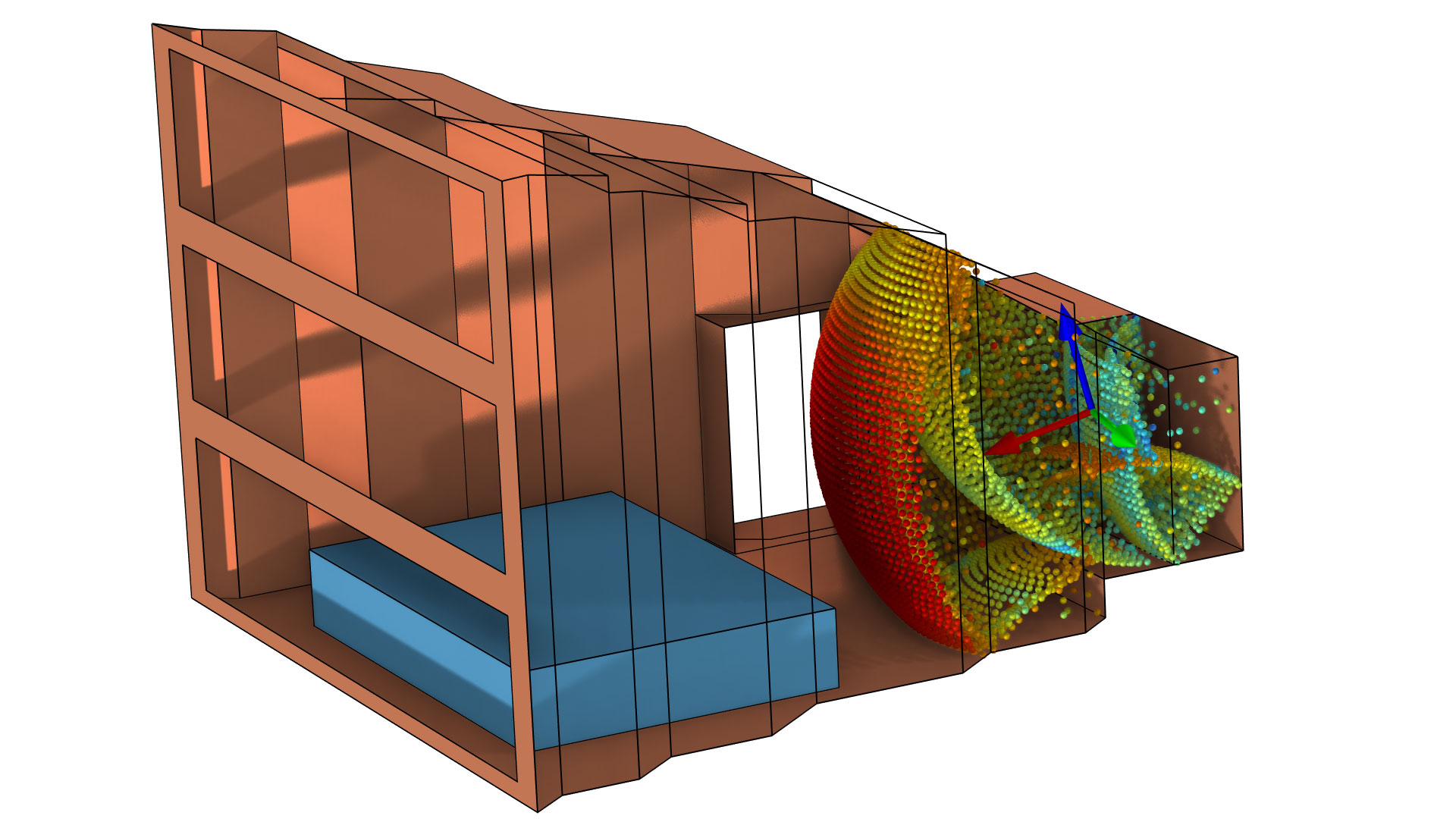
One-Family House Acoustics
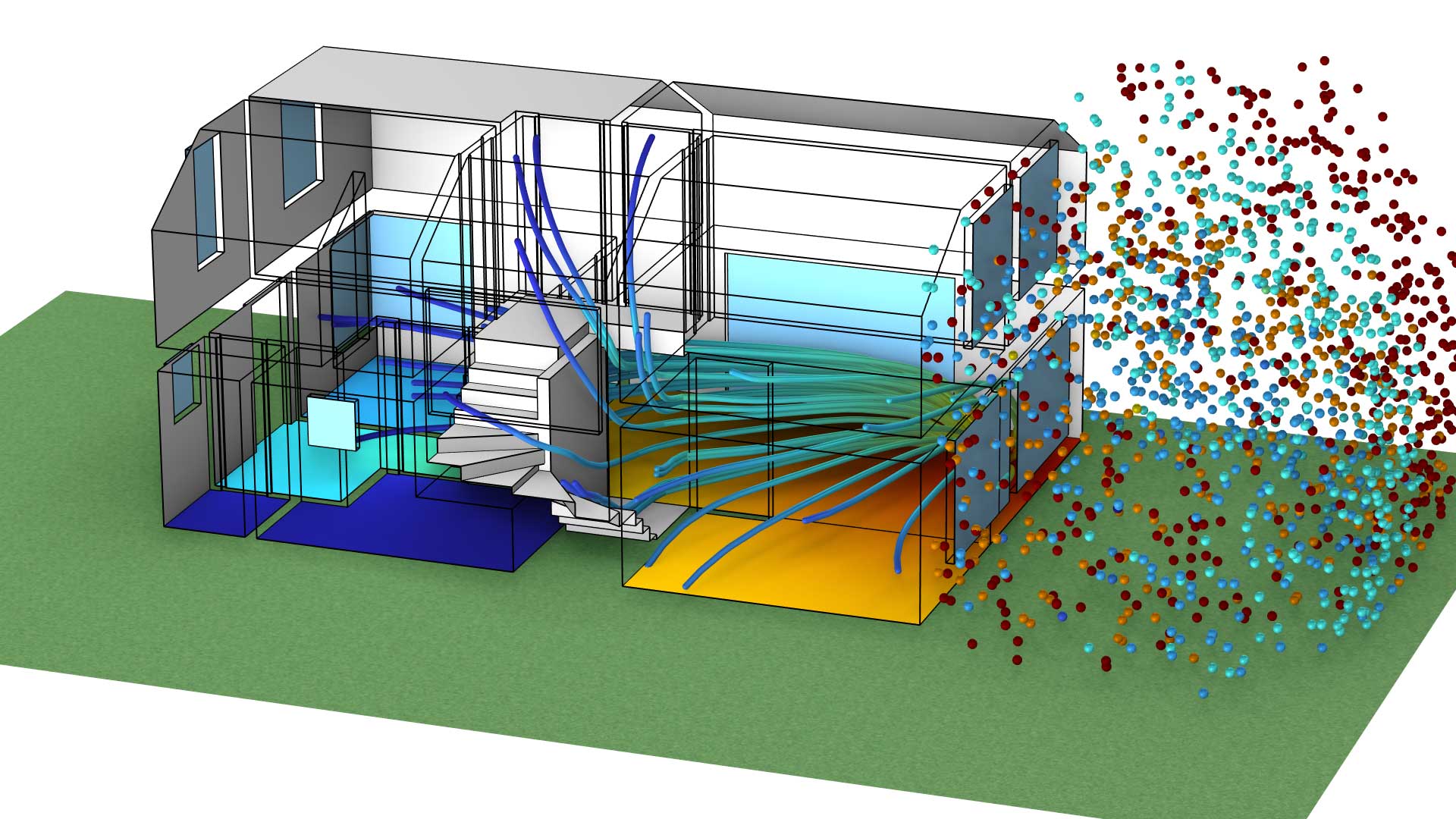
Application Library Title:
one_family_house
Download from the Application Gallery
Prestressed Micromirror Vibrations: Thermoviscous-Thermoelasticity Coupling

Application Library Title:
micromirror_prestressed_vibration
Download from the Application Gallery
Lumped Loudspeaker Driver Transient Analysis with Nonlinear Large Signal Parameters
Application Library Title:
lumped_loudspeaker_driver_transient
Download from the Application Gallery
Ultrasonic Flowmeter with Piezoelectric Transducers
Application Library Title:
flow_meter_piezoelectric_transducers
Download from the Application Gallery
Angle Beam Nondestructive Testing
Application Library Title:
angle_beam_ndt
Download from the Application Gallery
Loudspeaker Driver in a Vented Enclosure
Application Library Title:
vented_loudspeaker_enclosure
Download from the Application Gallery
Small Concert Hall Acoustics
Application Library Title:
small_concert_hall
Download from the Application Gallery
Type 4.3 Ear Simulator

Loudspeaker Driver in 3D - Frequency Domain Analysis
Topology Optimization of a Sound Partition Considering Acoustic-Structure Interaction
Electrostatic Speaker Driver
Simple Thermoacoustic Engine
Transient Sound Pressure Level
Balanced Armature Transducer
Transfer Matrix of a Tube and Coupler Measurement Setup
Ultrasonic Car Parking Sensor