Pipe Flow Module Updates
For users of the Pipe Flow Module, COMSOL Multiphysics® version 6.0 brings a new predefined friction coefficient for non-Newtonian flow in pipes and a new option for modeling T-junctions. Read more about these features below.
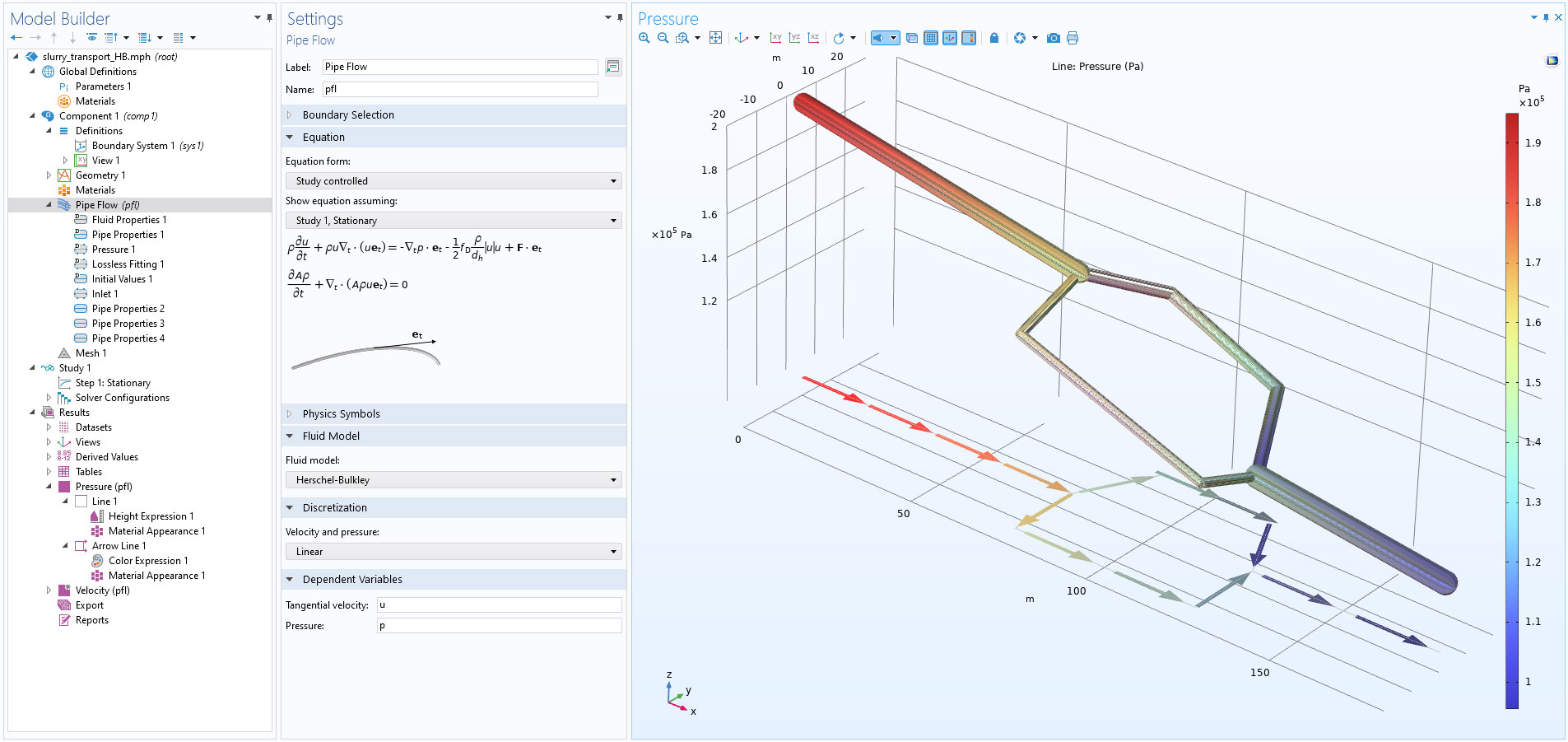
Non-Newtonian Flow in Pipes
A new Herschel-Bulkley fluid model is now available for the Pipe Flow interface. This model is often used to describe the rheological behavior of non-Newtonian fluids and is a generalization of the Bingham and Power law models. The Herschel-Bulkley model allows you to simulate flow of fluids exhibiting viscoplastic behavior. Practical examples of such materials are greases, colloidal suspensions, starch pastes, toothpaste, paints, and drilling fluids.

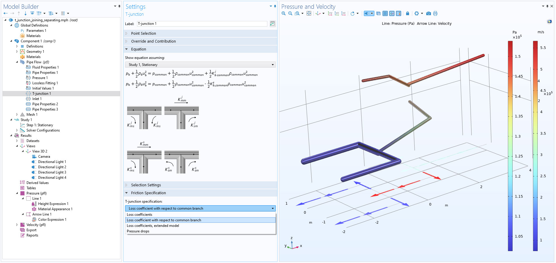
Improved Model for T-Junctions
The Pipe Flow interface now includes an additional option for the T-junction specification called Loss coefficient with respect to common branch, available in the T-junction node. This option automatically calculates the dimensionless loss coefficients accounting for a particular flow situation, for example, if the flow in the junction is joining or separating.
New and Updated Tutorial Models
COMSOL Multiphysics® version 6.0 brings new and updated models to the Pipe Flow Module.
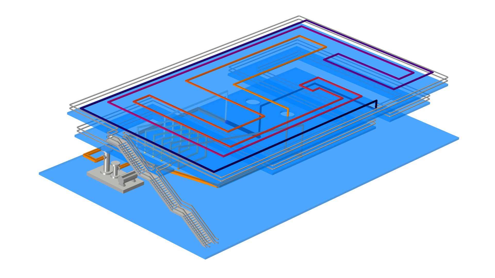
Topology Optimization of a District Heating Network

Application Gallery Entry:
district_heating_optimization
Download from the Application Gallery
Stress in Cooling Pipeline Network
Application Gallery Entry:
cooling_pipeline
Download from the Application Gallery