Structural Contact Modeling Guidelines
Structural contact modeling is a highly nonlinear problem. As surfaces come in and out of contact, load paths and stress states will abruptly change. The computational solvers in the COMSOL Multiphysics® software are designed to work with sufficiently smooth solutions, so solving such models is inherently challenging. To efficiently achieve a converged solution, most contact models will require some changes to the default model settings.
This article contains guidance for solving models that include structural contact and details that processes that should be followed to achieve a converged solution. To get the most out of this article you will need familiarity with structural modeling and the Form Union and Form Assembly geometry operations in the software. If you are unfamiliar with this topic, we recommend checking out the models included in the Bracket — Structural Mechanics Tutorials and reading the following article (includes videos): "The Usage of Form Union and Form Assembly".
The challenge of solving this class of problems arises from the fact that the displacement field,  , across the boundaries in contact is not continuous. To start, let's consider a normal contact mechanics case where any additional effects such as friction or adhesion are ignored and where stationary conditions are assumed.
| Strong Form | Weak Form |
|---|---|
 |
 |
Two new entities or quantities of interest are added to the governing equations, namely the gap function denoted by  and the contact pressure
  (positive under compression). As illustrated in the figure below, the gap function is defined as the geometric distance between the source,
  , and the destination,
  , boundaries. The search is performed in the direction of the destination spatial normal (this is not necessarily the smallest distance). Since the interpenetration of matter is not physical, the gap function must be a nonnegative quantity.
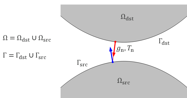
A schematic of the contact search and mapping between a source and destination boundary.
The contact pressure can be interpreted as the reaction force developed at the contact boundaries to ensure that the gap function remains nonnegative (strictly speaking, this is only true when adhesive forces are neglected). These two quantities add inequality constraints to the governing equations, and the contact problem becomes an optimization problem subject to the Karush–Kuhn–Tucker (KKT) conditions, which translates to the following set of constraints:

We've already described the first two constraints for the gap function and contact pressure. In the third constraint, if both surfaces are in contact,  , then the contact pressure is either zero (perfectly adjacent surfaces or mating boundaries) or positive (both surfaces are pushed against each other). Likewise, if the contact pressure is positive, then the gap function must be zero. The fourth constraint is called the persistency condition and states that if the gap function is changing, then the contact pressure must be zero.
In order to solve the contact problem described above, one needs to effectuate a contact search between the source boundary and the destination boundary. The purpose of this search is to detect points on the contacting boundaries that are in contact or may come into contact as well as to map quantities between such points. The contact search can be split into two steps: a broad search and a fine search. Three strategies are available for the broad search: Hierarchical, Distance Tracking, and Exhaustive. The fine search algorithm uses a ray-tracing strategy.
In COMSOL Multiphysics®, the Contact Method menu for Contact nodes include three options: Penalty (default), Augmented Lagrangian, and Nitsche. Unless explicitly stated, all of the recommendations in these guidelines are valid for all three methods. Please refer to the "Contact Analysis Theory" section of our documentation for a detailed discussion of these methods.
General Guidelines for Structural Contact Modeling
Creating Contact Pairs
In general, the finalization of your model geometry should be completed with the Form Assembly node if it contains parts that are adjacent to each other and have mating boundaries. Models will include a Form Union node under the Geometry node by default, which can be changed by choosing the Form an assembly option in the Form Union/Assembly menu. In the same menu, select Create Pairs and then select the Contact Pair option. This will automatically create contact pairs between mating boundaries of objects — any unwanted contact pair can be deleted later.
See "The Usage of Form Union and Form Assembly" for more information.
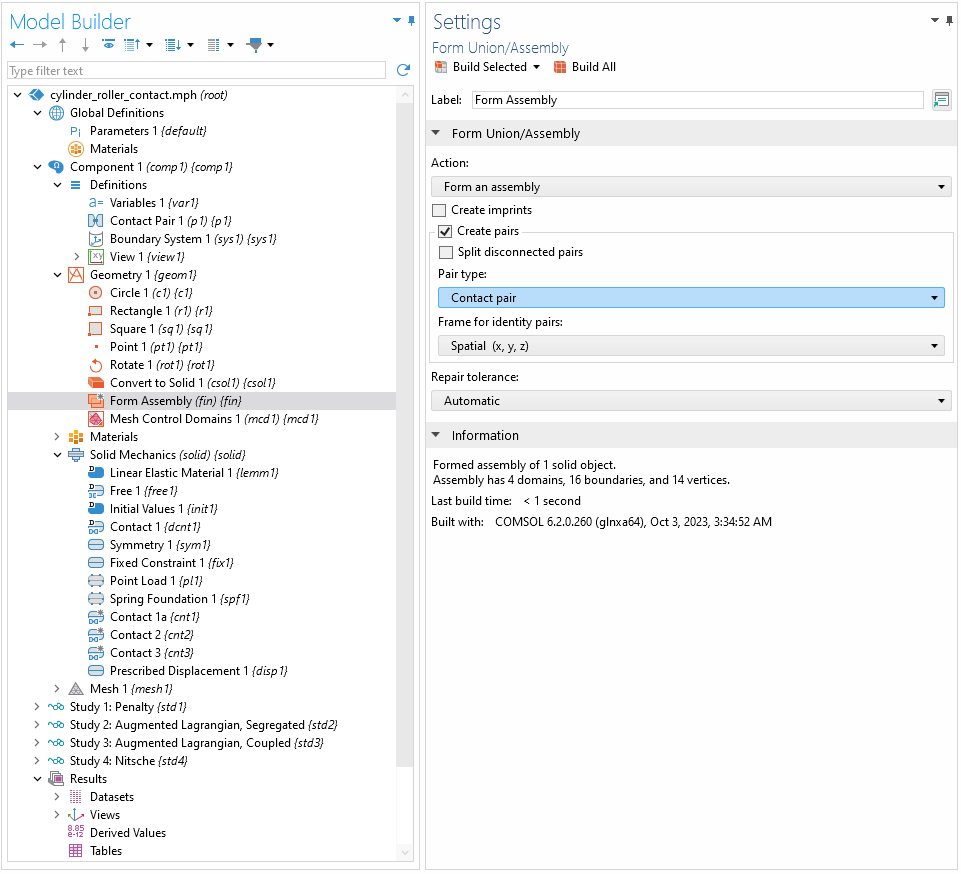 The Form Union/Assembly window with the Create pairs and Contact pair checkboxes selected.
The settings for the Form Union/Assembly node, where the action is set to Form an Assembly , the Create Pairs checkbox is selected, and the pair type is set to Contact pair.
The Form Union/Assembly window with the Create pairs and Contact pair checkboxes selected.
The settings for the Form Union/Assembly node, where the action is set to Form an Assembly , the Create Pairs checkbox is selected, and the pair type is set to Contact pair.
For boundaries that are not initially in contact but will come into contact during the simulation, you will need to manually create contact pairs between the boundaries. The figure below illustrates when a Contact Pair coupling under the Definitions node needs to be manually created. Note that the use of finalized assemblies in multiphysics models is not supported by all built-in multiphysics couplings, and support should be verified on a case-by-case basis.
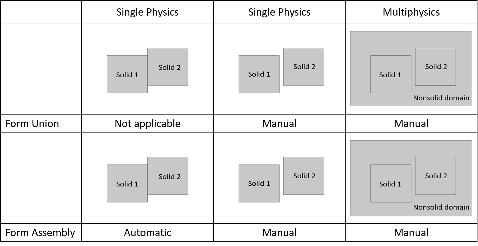
This table illustrates when a Contact Pair can be added to the model and whether it can be created automatically or if it needs to be manually added.
Note: If you anticipate contact between any sharp corners and surfaces in the model, you should modify the geometry such that a sharp corner is replaced with a rounded boundary — a fillet. The fillet radius can be very small, and that surface will need to be meshed quite finely.
All contact pairs, both manually and automatically created, are defined at: Component > Definitions > Contact Pair.
Within the Contact Pair node, select the boundary of the stiffer part under the Source Boundary menu. If the parts have a similar stiffness, set the concave parts as the source and the convex parts as the destination. Use the Swap source and destination button for this. For efficiency, include in each contact pair only those boundaries that have the possibility of coming into contact.
It is important to know that, for performance reasons, the standard formulation for the Contact Pair feature can be viewed as a biased (or unsymmetric) formulation in the sense the contact forces are added on one side — the destination boundary. However, as we shall see in the "Mesh" section below, this formulation imposes requirements on the mesh size of both sides. Note that it is also possible to set up an unbiased (or symmetric) formulation by using the same selection for the source and destination boundaries in a Contact Pair. An unbiased formulation is typically needed when modeling self-contact or when it is not self-evident which boundaries should be the source or destination.
The Hierarchical setting is the default option for the Search method setting because it can handle large models efficiently. You do not need to change this setting unless you encounter problems with the mapping. In that case, you can try the Distance Tracking option, which may give more accurate results. The Exhaustive method is the most reliable but also the most expensive in terms of memory and computation time. You should use it only as a last resort.
If it is expected that there will be little sliding between the contacting boundaries (such as in a shrink fit or when two parts are bolted together), then go to the Contact Pair > Advanced settings and change the mapping method to Initial configuration. The mapping between the source and destination boundaries will be computed only once, based on the initial positions of the domains, which leads to faster and more stable convergence.
Note: In general, multiple Contact Pair nodes are only needed if they have different settings or if different settings are needed in the physics.
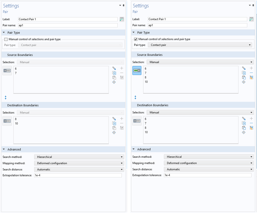 Two Settings windows for the Pair feature showing different boundary selections.
Left: The settings for the Contact Pair node, where the selection lists for the source and destination boundaries are different, and thus a biased formulation is used. Right: The settings for the Contact Pair node, where the selection lists for the source and destination boundaries are the same, and thus an unbiased formulation is used.
Two Settings windows for the Pair feature showing different boundary selections.
Left: The settings for the Contact Pair node, where the selection lists for the source and destination boundaries are different, and thus a biased formulation is used. Right: The settings for the Contact Pair node, where the selection lists for the source and destination boundaries are the same, and thus an unbiased formulation is used.
Physics
By default, a Contact node is added to the structural physics interface (e.g., the Solid Mechanics interface). The default Contact node will include all contact pairs in the Definitions node. However, if needed, additional Contact nodes can be added to the model if they have different settings. The Solid Mechanics and Multibody Dynamics, Shell, Layered Shell, and Membrane interfaces provide support for contact modeling. Contact modeling in thin structures requires the options under the Contact Surface menu of the corresponding Contact node to be correct. The correct option, Top or Bottom, depends on the physics interface normal, not the geometry normal. The contact will not work unless the physics normals are pointing toward each other. Moreover, it is possible to model contact between different physics interfaces, such as between the Solid Mechanics and Shell interfaces.
Within the Contact feature, select either the Penalty, Augmented Lagrangian, or Nitsche option as the contact method. The Penalty method is relatively less accurate but more robust and will require less solver tuning, making it preferable for multiphysics problems and time-dependent models. The Penalty method must be used when modeling adhesion. The Augmented Lagrangian method is the most accurate method but has a higher computational cost and will require more fine-tuning to converge. The Nitsche method (supported by the Solid Mechanics and Multibody Dynamics interfaces only) can be viewed as an enhancement of the penalty method and is intended as an alternative to the Augmented Lagrangian method for problems where the penalty method lacks sufficient accuracy. Also note that the Penalty method has the advantage that no special solver is required, which makes it easier to set up multiphysics problems and time-dependent studies.
Generally speaking, the available methods can be sorted as follows in terms of robustness: penalty, Nitsche, segregated augmented Lagrangian, and fully coupled augmented Lagrangian. Unfortunately, the robustness is inversely proportional to the method accuracy, computational cost, and amount of effort to make the model converge. If you are not interested in an accurate contact pressure field distribution, but in the structural stiffness of the global system, then the Penalty or Nitsche method should suffice. However, the Nitsche method is typically recommended when modeling self-contact or large deformation problems with hyperelasticity material models. The Augmented Lagrangian method is typically used when an accurate contact pressure distribution is of interest or when modeling larger deformation with plasticity, such as for die-forming applications.
When running into convergence problems, manual tuning of the penalty factor may be needed, though this should only be done after all of the other recommendations in these guidelines are followed. Before fine-tuning this factor, it is important to understand its interpretation: The penalty method represents the stiffness of a spring between the contact surfaces. A larger value reduces the unphysical penetration but worsens the numerical condition of the stiffness matrix and makes the method less robust. A too-small value can cause a violation of the contact condition.
The convergence behavior of the augmented Lagrangian method is influenced by the penalty factor, but the accuracy of the solution is not impacted. The influence of this parameter differs for segregated and coupled methods. When using the segregated method, the penalty factor controls how “hard” the interface surface is during the iterations but does not directly affect the converged results. The Contact Pressure Penalty Factor menu includes three tuning options associated with the preset Penalty Factor Control option. The tuning options include Stability (default), Speed, and Bending. If the contacting parts are in contact at the start of the simulation, then Speed is the preferred setting. When using the coupled method, the penalty factor affects the equation structure, and the solution is less sensitive to its value. However, adjusting the penalty factor can enhance the convergence properties.
When using the Nitsche method, the penalty factor acts as a stabilization parameter that affects robustness without heavily impacting the accuracy. The optimal value depends on the formulation, where the Skew-symmetric and Incomplete (default) formulations are more robust than the Symmetric option.
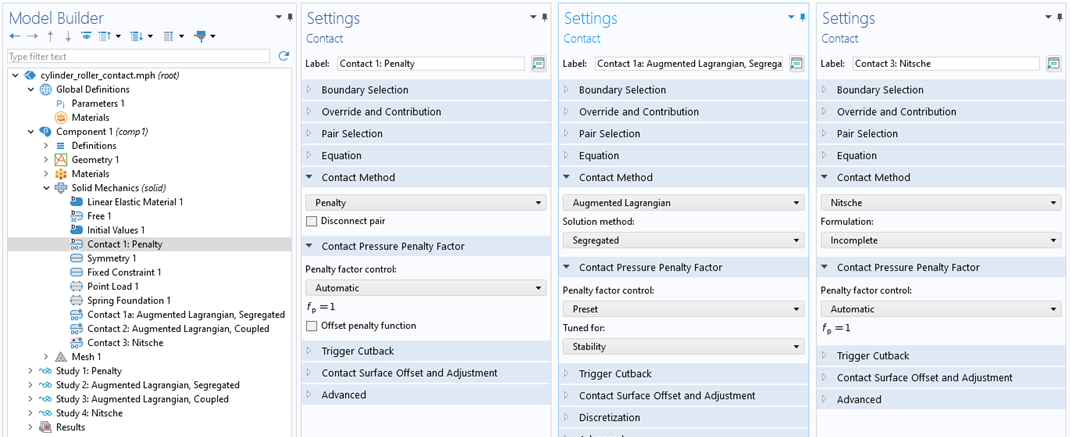 The Model Builder with the Contact node highlighted and three Settings windows for the Contact feature with different settings in each.
Settings windows for the Contact node showing the contact method set as Penalty, Augmented Lagrangian with Segregated as the solution method, and Nitsche.
The Model Builder with the Contact node highlighted and three Settings windows for the Contact feature with different settings in each.
Settings windows for the Contact node showing the contact method set as Penalty, Augmented Lagrangian with Segregated as the solution method, and Nitsche.
If one part is significantly stiffer than the others, its deflections will be relatively negligible, and it can often be considered as rigid. This is a simplifying assumption that will make the problem easier to solve. To apply this assumption, add a Prescribed Displacement boundary condition to the rigid domain. Select the Prescribed option and enter a value of 0 for the displacement in the assumed rigid directions. The rigid domains can have a very coarse mesh on any planar boundaries; however, any curved contact boundaries will still need to be finely meshed. The rigid part should be the source in the Contact Pair node. The mesh on the boundaries of the deformable domains will need to be fine enough to give a good resolution of the contact patch and stress state. Alternatively, one could also assign a Rigid Material feature to this domain or remove it from the physics selection. Note that in the latter case, the contact boundary requires a mesh even though it is not part of any physics.
It is better to have a Prescribed Displacement constraint on all domains that will come into contact in the model. This will be easier to solve than cases where the domains include applied loads, forces, and contact conditions but are otherwise unconstrained. If it is possible to reformulate your problem such that there is some initial constraint on all domains, do so.
If you must model a domain that is initially unconstrained, you have two options:
- Add a Spring Foundation feature to these unconstrained, deformable domains (or to the boundaries of these domains). The magnitude of this spring constant is initially set at a very high value — high enough such that the deformations are negligible due to the initially applied loads. As this spring constant is reduced to zero, the domain will gradually relax into its deformed state due to contact and applied loads.
- Add the Stabilization subnode to suppress rigid body motion related to such unconstrained parts. This feature can be seen as an automated version of the Spring Foundation feature, and three stabilization techniques are available: Adjacent domains, Contact boundaries and, Contact Pairs. The stabilization works by connecting springs to the ground for those geometric entities. When Contact Pairs is selected from the list, springs are instead added between the source and destination of the contact pairs of the parent Contact node.
If you are solving a stationary (steady-state) model, you will want to ramp the prescribed displacements, loads, and stiffnesses of any spring foundations during the solution. Introduce a new Global Parameter (name it, e.g., RampFactor) and multiply all loads, displacements, and stiffnesses by this factor. The ramping of this parameter will be defined within the study settings (see the section below). For instance, the ramping of spring constants used for spring foundations on unconstrained domains should begin at the peak value of spring stiffness and then ramp down to zero. In this case, a nonlinear decrease of spring stiffness is recommended. Using the parameter RampFactor that ranges linearly from 0 to 1, a spring foundation with spring constant kz in the Z direction can be introduced where kz = k0*(1-RampFactor)*2^(-RampFactor*10), and similarly in any other directions that need to be restrained. The peak value of spring stiffness, k0, should be chosen such that the displacement due to the full applied load is about equal to the element size of the contacting boundaries.
When spring foundations and applied loads are in a single model, the applied loads should be ramped up linearly at the same time as the spring constants for the spring foundations are ramped down nonlinearly using the above expression (shown in the plot below).
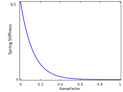
Spring foundation stiffness function: The stabilization stiffness is ramped down nonlinearly and is zero when RampFactor is equal to 1.
If you are solving a time-dependent (transient) model, make sure that all prescribed displacements, loads, and stiffnesses of any spring foundations are time dependent and ramped over a physically reasonable time span, not just for the solid mechanics physics, but for all other physics that are included if it is a multiphysics model. For more information on this, see the following Learning Center article: Modeling Step Transitions.
If you are solving a transient model but do not want to consider inertial effects (e.g., if you do not want to model the vibrations of the structure), then go to the Solid Mechanics interface, and in the Structural Transient Behavior settings, select Quasi-static, which will solve much more quickly. Note that specialized versions of the contact penalty factor for the Penalty and Augmented Lagrangian methods are available for dynamical contact problems. These formulations add a viscous penalty factor contribution to the governing equations that constrain the gap rate to zero (i.e., the persistence condition), and one must provide the Characteristic time of the contact. As a rule of thumb, it should be of the order of the contact event duration, but the best choice must be decided on a case-by-case basis.
Mesh
It is important to mesh the contacting boundaries sufficiently finely. Manual meshing will need to be used. The contacting boundaries should be meshed finely enough to give good resolution of the contacting area. The destination boundary of the contact pair must be meshed finer than the source boundary, by at least a factor of two. Curved surfaces will need to be meshed more finely than flat surfaces. This is because the default algorithm is asymmetric: The points on the destination side connects to the source side and not vice versa. With a coarse mesh on the destination side, a large portion of an element (or even a whole element) on the source side could be without connection to the destination. Failing to follow these guidelines can cause unphysical oscillations in the contact pressure.
If the source boundary is rigid, there are no requirements on the mesh size of the destination boundary. However, the mesh in the source boundary should be fine enough to resolve the curvature of the geometry. In the case of a symmetric formulation (same selection for source and destination), a uniform mesh element size along the contacting boundaries is recommended.
Study Settings
When solving a Stationary study, you will want to ramp up the prescribed displacements, loads, or spring foundations on unconstrained domains. First introduce a Global Parameter that multiplies all displacements, loads, and stiffnesses, such as RampFactor. Ramp this parameter via the Auxilliary sweep option within the Stationary study step settings.
The ramping of applied loads and displacements should begin from a value very close to zero, at which there is negligible or even no contact, and should ramp up linearly to the maximum value. For example, the image below shows RampFactor starting at a value of 0.001 and then increasing from 0.1 to 1 in increments of 0.1. By default, the continuation method will be used, which uses the solution from the previously solved step as the initial condition for the next step, thereby easing convergence. (See the following Learning Center article for additional information: "Improving Convergence of Nonlinear Stationary Models"). The number of increments may need to be quite large, and you will want to monitor at what values of the ramping factor there is slow convergence of the solver. Use more increments when the convergence is slow.
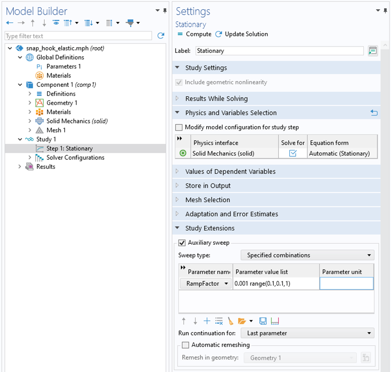 The Model Builder with the Stationary study step highlighted and the corresponding Settings window with the Auxiliary sweep checkbox selected.
The settings for the Auxiliary sweep option in the Study Extensions section.
The Model Builder with the Stationary study step highlighted and the corresponding Settings window with the Auxiliary sweep checkbox selected.
The settings for the Auxiliary sweep option in the Study Extensions section.
Solver Settings
Use the default suggested direct solver rather than the iterative solver whenever possible. The iterative solver will require less memory, but convergence is usually much slower.
For stationary models with an auxiliary sweep over a ramping parameter, the default behavior is to use the continuation method. Within the Settings window for the Parametric node, selecting the Constant option for the Predictor setting will make the convergence more robust but slower. This setting is shown in the screenshot below.
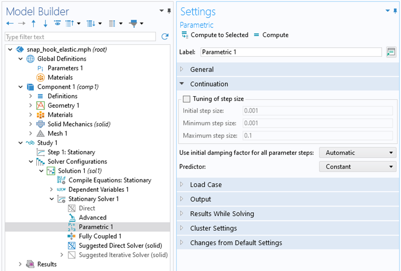 The Model Builder with the Parametric node highlighted and the corresponding Settings window.
The auxiliary sweep parametric settings.
The Model Builder with the Parametric node highlighted and the corresponding Settings window.
The auxiliary sweep parametric settings.
When using the augmented Lagrangian formulation with Segregated selected as the solution method, the default solver configuration uses a segregated approach, where the contact pressures (and friction forces, if friction is included) are solved in a separate lumped or segregated step. This should not be changed. If you have to modify the solver sequence, this separate segregated group should be kept and solved for after the displacements.
When using the augmented Lagrangian formulation, it is necessary to manually scale the variables in a contact problem. If you cannot estimate the contact pressure before the solution, you may need to perform the analysis in two passes, where you first compute an estimate of the contact pressure using the penalty formulation. The scaling of the contact pressure is used when checking the convergence, so if a too-high value is used, there is a risk that the results are not correct. The default scaling value is set to a typical metal-to-metal contact. For further information on scaling dependent variables, please see the following Learning Center article: "Manually Setting the Scaling of Variables".
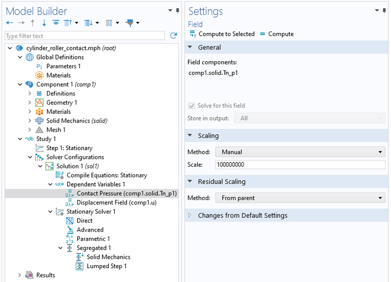 The Model Builder with the Field node for Contact Pressure highlighted and the corresponding Settings window.
The Settings window for the contact pressure scaling when the augmented Lagrangian method is used.
The Model Builder with the Field node for Contact Pressure highlighted and the corresponding Settings window.
The Settings window for the contact pressure scaling when the augmented Lagrangian method is used.
Modeling of Contact with Friction
Modeling friction will often increase the computation time significantly, so if you can reasonably ignore friction, do so. Friction usually only causes minor local effects, and friction coefficients are difficult to obtain with any accuracy, so this simplification is practically justified. If, however, there are significant shear stresses on contact boundaries, or if frictional dissipation is important, friction must be included.
If your contact simulation does involve friction, set up and solve the problem without friction first. Once the appropriate solver settings have been found, add friction and re-solve. Contact problems with friction should always be solved incrementally using a parametric or time-dependent solver since the development of friction forces is history dependent.
Note: Friction can sometimes be added to initially unconstrained assemblies. The tangential force can help maintain stability and avoid rigid body motion.
Multiphysics Contact Modeling
In some contact problems, there is some kind of flux (or transport) of a quantity from one solid domain to another through the contact zone. Classical examples are heat flux, electric current, or moisture transport. To solve this class of multiphysics problems, we need to know what happens at the boundary where the contact occurs or does not occur. By default, whenever in contact, continuity of field and flux is assumed unless a contact node is included in the heat transfer or electromagnetics physics interface (e.g., the Pair Electrical Contact or Thermal Contact interface). These contact nodes capture the "resistance" to transfer these quantities due to asperities and interstitial fluid in the contact zone. Note, however, that these contact nodes are not available for all physics interfaces and should be checked on a case-by-case basis. In the case of out-of-contact surfaces, a fallback boundary condition is applied to all parts of the boundaries currently included in the boundary selection list of the Contact node. It is possible to overwrite the default Applicable Pair Region option when Advanced Physics Options is enabled from the Show More Options dialog. An example with this option enabled is shown below with the Heat Flux feature.
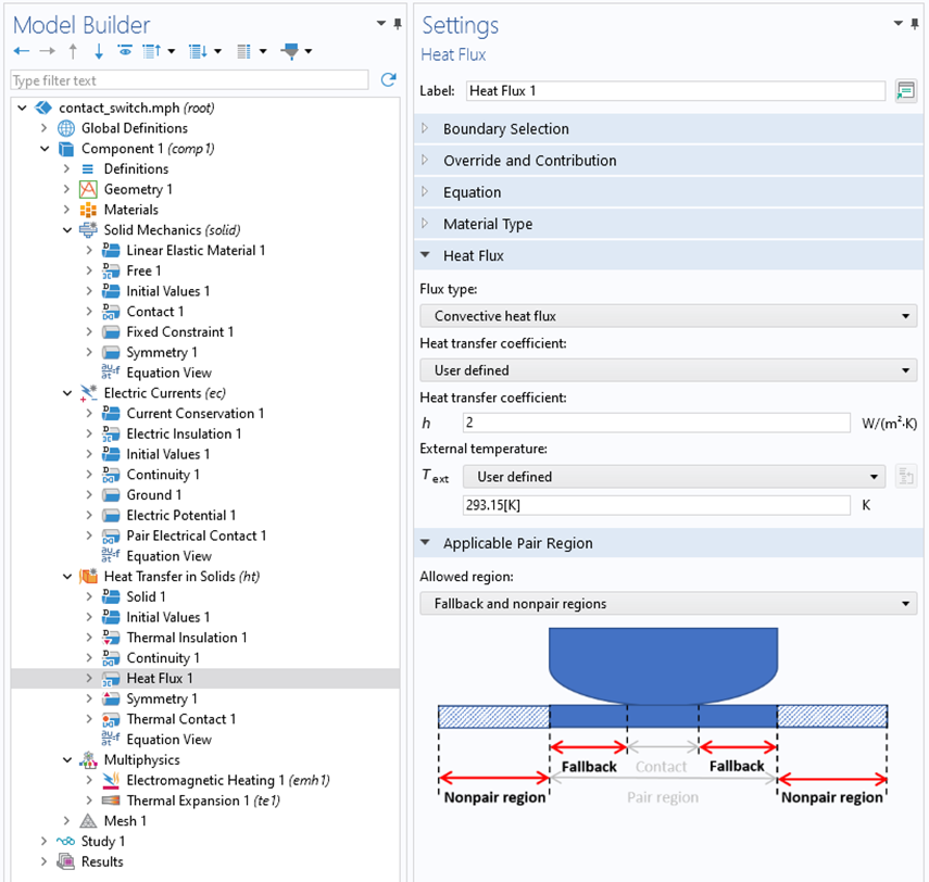 The Model Builder with the Heat Flux node highlighted and the corresponding Settings window.
The settings for the fallback convective heat flux.
The Model Builder with the Heat Flux node highlighted and the corresponding Settings window.
The settings for the fallback convective heat flux.
When a field exists in the gap between the domains controlled by the structural physics interface, then additional measures need to be taken to successfully run the simulation. Common applications involve fluid–structure Interaction (FSI), electromechanical force, or magnetomechanics multiphysics couplings. If contact is established, the mesh in the original gap between the source and destination boundaries will collapse. This must be avoided since the arbitrary Lagrangian–Eulerian (ALE) formulation used to deform the nonsolid field domain requires that the connectivity of the mesh remains unchanged during the mesh deformation, which means that topological changes in the geometry are not allowed. One way to fix this problem is to adjust the contact settings by adding an offset to either the source boundary, the destination boundary, or both (see the Settings window below). This will allow the contact forces to be transferred without closing the gap completely, but there will be a very small amount of flux passing through the gap.
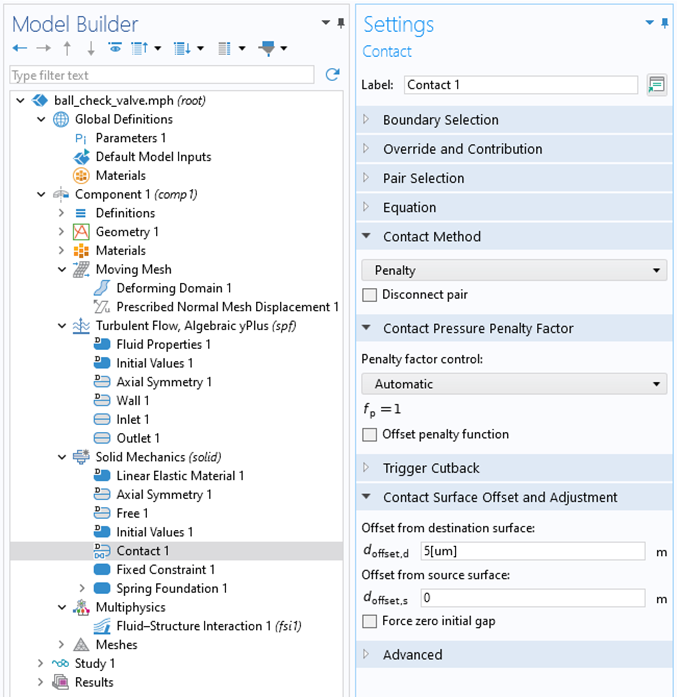 The Model Builder with the Contact node highlighted and the corresponding Settings window.
Example of settings in the Contact Surface Offset and Adjustment section.
The Model Builder with the Contact node highlighted and the corresponding Settings window.
Example of settings in the Contact Surface Offset and Adjustment section.
Contact Modeling Checklist and Further Learning
Below, you will find questions that we recommend considering when modeling contact:
- Do you have contact between sharp corners? If so, add fillets.
- Are the source and destination boundary selection lists following the recommendations based on the stiffness and curvature of the contact parts?
- Are you ramping displacements/loads boundary conditions using an auxiliary step or a time-dependent function?
- Did you add any stabilization when modeling a quasistatic or stationary problem with a load-driven boundary condition?
- Is your mesh at least twice as fine on the destination side when compared with the source side?
- Did you include an offset when modeling a multiphysics problem where a field exists in the gap between the two contact boundaries?
To learn more about contact modeling, check out the "Structural Mechanics Module User's Guide" in the documentation and navigate to "Structural Mechanics Modeling" > "Contact Modeling".
Submit feedback about this page or contact support here.