COMSOL Multiphysics^® 6.1 Release Highlights

Wave Optics Module Updates

For users of the Wave Optics Module, COMSOL Multiphysics^® version 6.1 introduces dielectric scattering functionality, the Linearly polarized plane wave background field feature in 2D axisymmetry, and new tutorial models. Read about these updates and more below.

Dielectric Scattering with the Electromagnetic Waves, Boundary Elements Interface

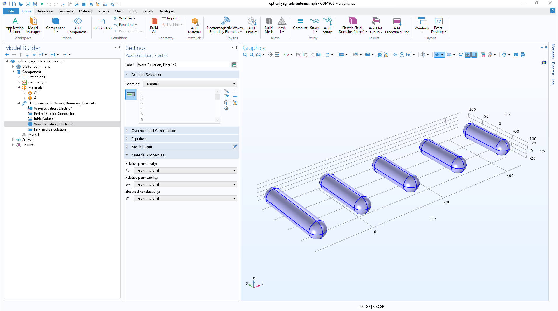
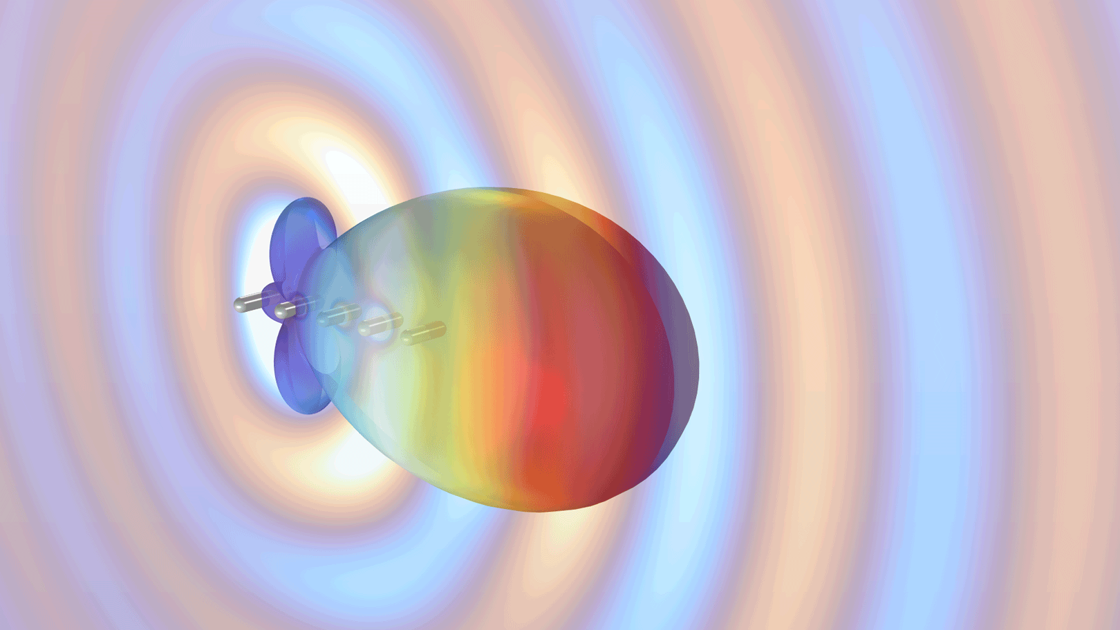
The interaction of electromagnetic waves with dielectric objects is now supported for the boundary element method, including the calculation of the associated far-field scattering properties. The new functionality is available in the Electromagnetic Waves, Boundary Elements interface. It requires adding a Wave Equation, Electric node to each dielectric scatterer domain. Furthermore, a Far-Field Calculation node can be added to evaluate far-field quantities such as the scattering amplitude. You can see this feature demonstrated in the new Optical Yagi-Uda Antenna model.

A second Wave Equation, Electric node is selected in the Model Builder window, representing aluminum scatterers. The first Wave Equation, Electric node represents the infinite air domain.

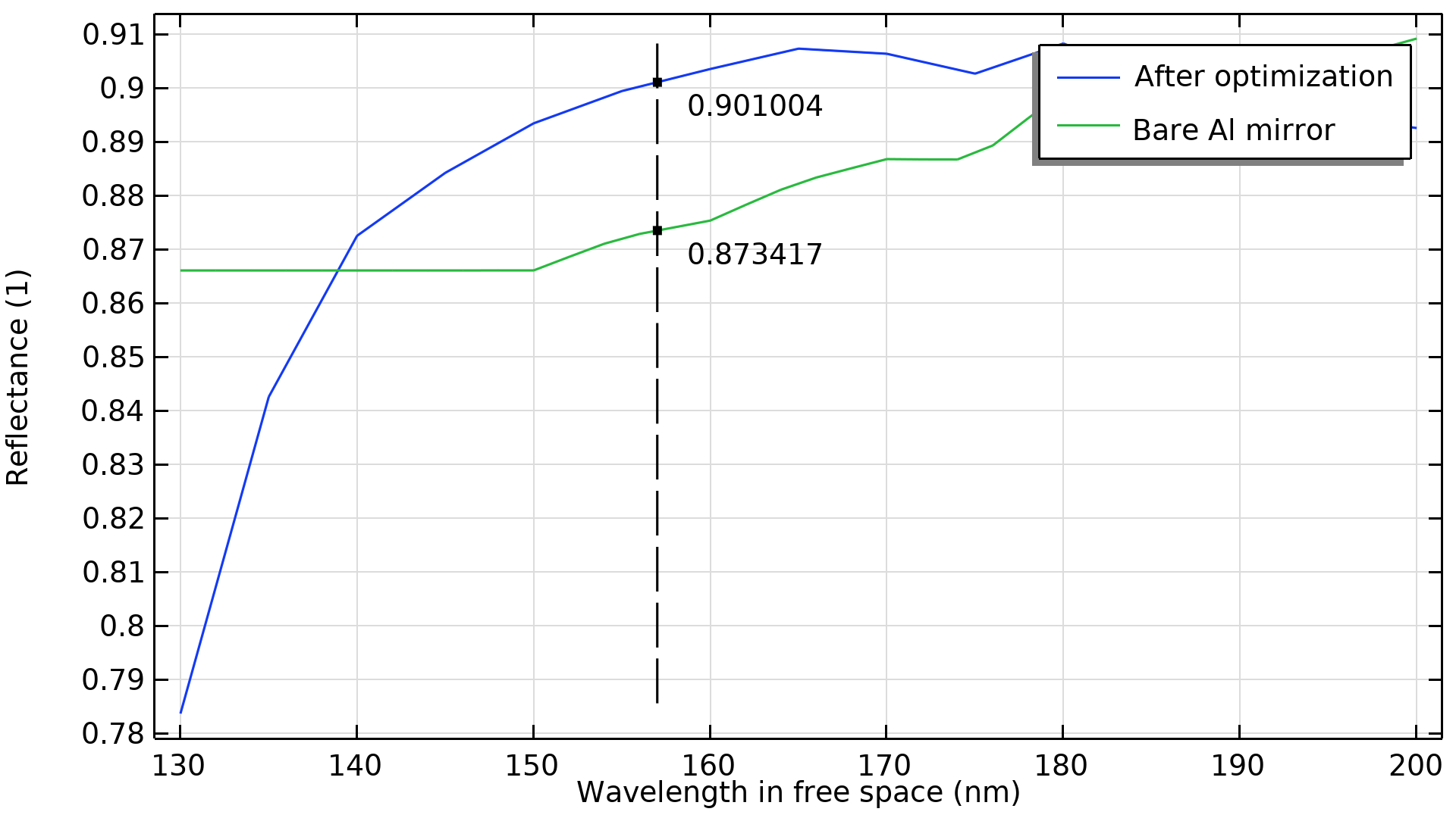
Layered Impedance Boundary Condition

New functionality enables you to model multiple thin layers on top of a substrate with small skin depth. This includes, for example, modeling thin dielectric coatings on a metal surface. Such thin layers can be described using the Layered Impedance Boundary Condition feature, available in the Electromagnetic Waves, Frequency Domain interface. It requires combining a Layered Material in the global Materials and a Layered Material Link in the Materials node. You can see this feature demonstrated in the new Enhanced Coating for a Microelectromechanical Mirror model.

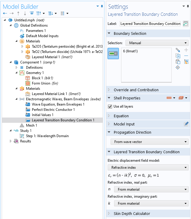
Layered Transition Boundary Condition

The Layered Transition Boundary Condition in the Electromagnetic Waves, Frequency Domain interface has now also been added to the Electromagnetic Waves, Beam Envelopes interface. The Layered Transition Boundary Condition has also been updated to include all material models that are available for the Transition Boundary Condition, which simplifies the definition of the material parameters for the boundary condition.

Linearly Polarized Plane Wave Background Field in 2D Axisymmetry

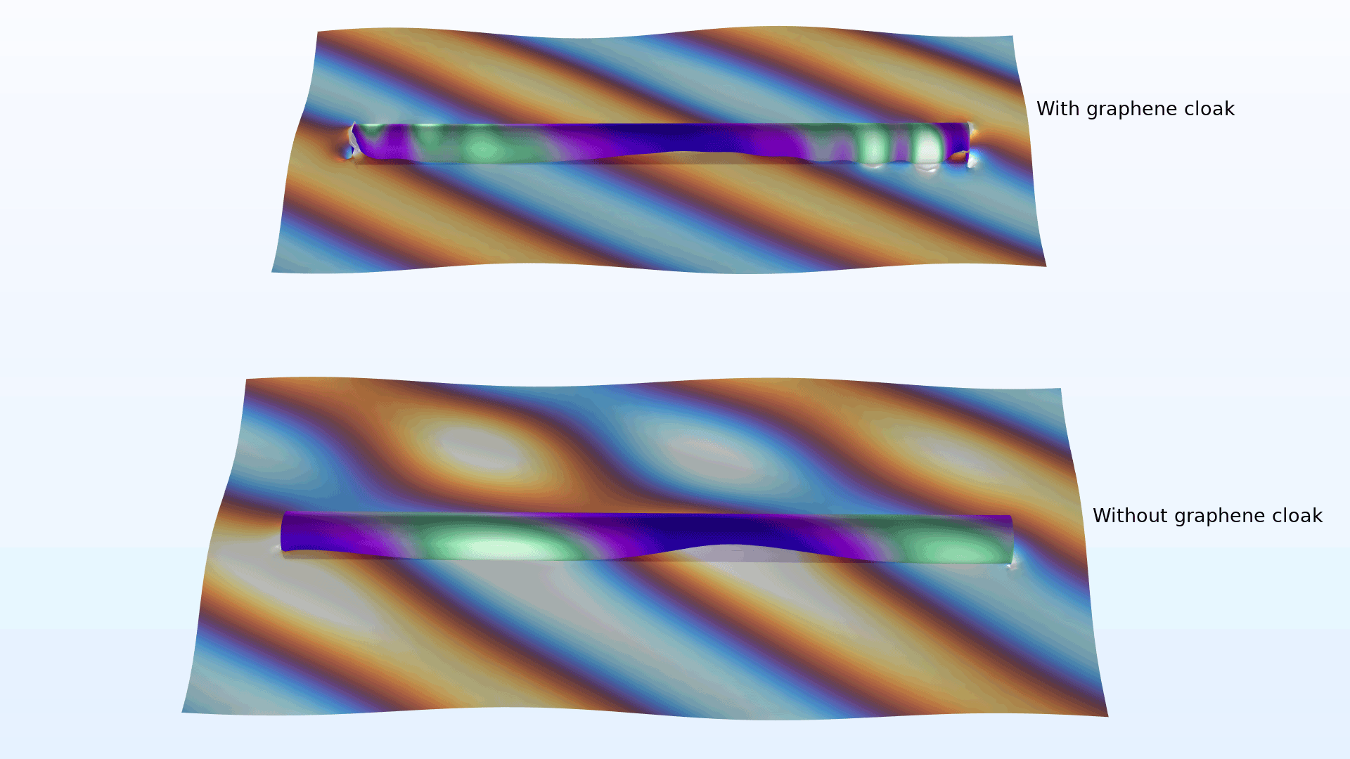
The Linearly polarized plane wave background field type with arbitrary polarization and incident angle is now available for 2D axisymmetry and utilizes an expansion method. It is suitable for modeling the scattering of bodies of revolution under plane-wave excitation. When compared with modeling the same problem in 3D, the 2D axisymmetric model uses significantly less memory and time, especially for electrically large scatterers, and facilitates using a denser mesh for improved accuracy. When using the Linearly polarized plane wave background field in 2D axisymmetry, an auxiliary sweep of the azimuthal mode number is automatically added. To construct the full solution, summing over the contribution from each azimuthal mode is required in postprocessing. You can see this feature demonstrated in the new Cloaking of a Cylindrical Scatterer with Graphene (Wave Optics) model.

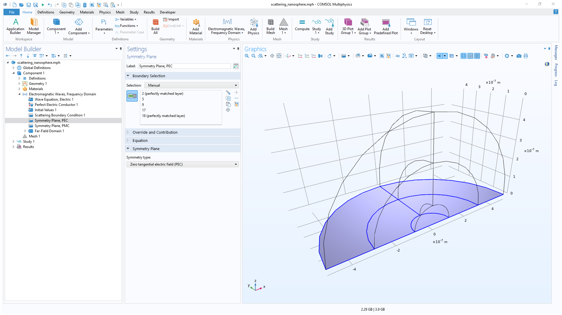
New Easy-To-Use Symmetry Plane Feature

The Symmetry Plane feature simplifies the definition of perfect electric conductor (PEC) and perfect magnetic conductor (PMC) symmetry planes. This feature is used instead of the Perfect Electric Conductor and Perfect Magnetic Conductor boundary conditions when reducing the model size from symmetry considerations. Furthermore, the information about the type and location of the Symmetry Plane features are used when calculating far fields and when defining analytical Port mode fields and Lumped Port impedance. You can see this new feature in the following models:

• scattering_nanosphere
• self_focusing
• fabry_perot_resonator

The use of Symmetry Plane nodes in the Optical Scattering off a Gold Nanosphere tutorial model.

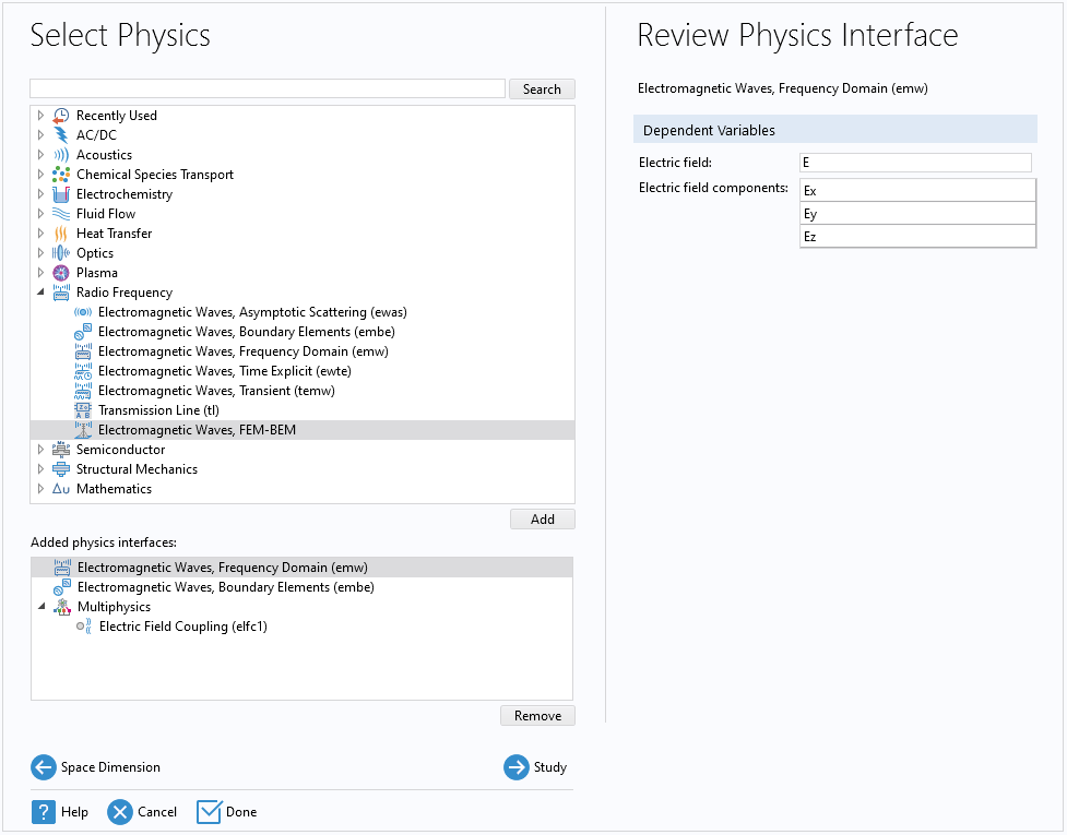
Finite Element Method (FEM)–Boundary Element Method (BEM) Multiphysics Coupling

A new FEM–BEM coupling feature simplifies the setup of hybrid FEM–BEM models for electromagnetic waves. This is available in the Model Wizard as an Electromagnetic Waves, FEM-BEM multiphysics interface, which combines the Electromagnetic Waves, Frequency Domain and Electromagnetic Waves, Boundary Elements interfaces with a new Electric Field Coupling multiphysics coupling feature.

Weak Formulation Port Option

When expanding the electric field on a port boundary, the new Weak port formulation adds a scalar dependent variable for the expansion coefficient (the S-parameter) and then solves for the S-parameters and the tangential electric field on the boundary using only a weak expression. Since no constraints are used, this formulation completely removes the constraint-elimination step when solving. This new port formulation replaces the constraint-free port formulation that was introduced in version 6.0.

You can see this new port formulation in almost all port-based tutorial models, such as:

• optical_ring_resonator_3d (new)
• plasmonic_wire_grating
• hexagonal_grating

Covariant Formulation in 2D Axisymmetry

In the 2D axisymmetric formulation, it is beneficial to formulate the out-of-plane dependent variable as

,

which is referred to as the covariant formulation. Here, Ψ is the dependent variable and is the radial coordinate. The out-of-plane electric field component is thereby calculated as

The covariant formulation has better performance in terms of numerical stability and accuracy. Compared to previous versions, eigenfrequency simulations can return fewer eigenfrequencies; however, the returned solutions have better accuracy, and there are many fewer spurious solutions returned.

This formulation is used for all study types except Mode Analysis and Boundary Mode Analysis and can be viewed in the following models:

• cylinder_graphene_cloak
• step_index_fiber_bend
• vertical_cavity_surface_emitting_laser
• whispering_gallery_mode_resonator

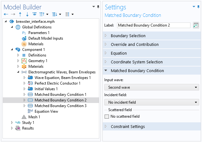
No Incident Field Option For Scattering and Matched Boundary Conditions

For the Scattering Boundary Condition and Matched Boundary Condition in the Electromagnetic Waves, Beam Envelopes interface, there is now a default option for the Incident field parameter: the No incident field value. You can use this option if there are only outgoing waves at the boundary. The following existing models highlight this option:

• brewster_interface
• beam_splitter
• fabry_perot_resonator

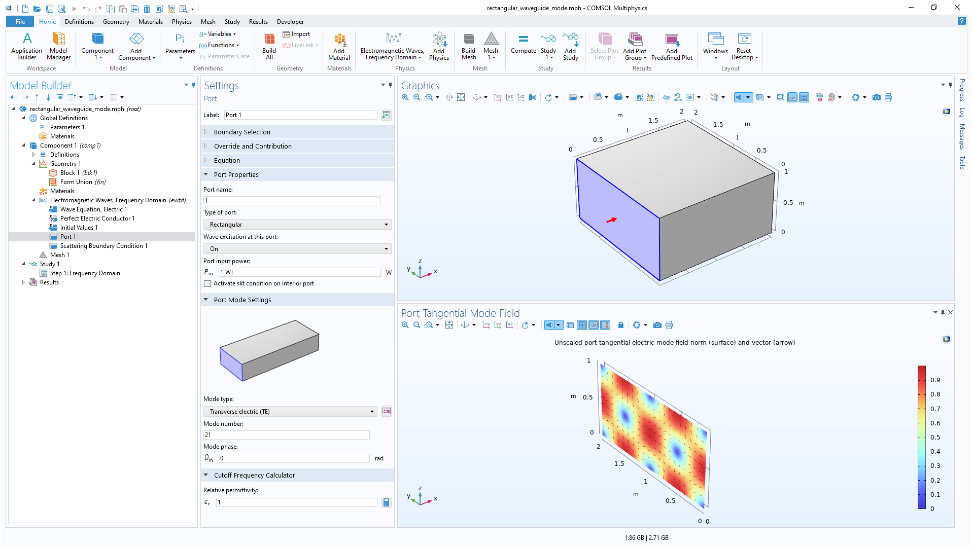
Plotting Analytical Port Mode Field Before Computation

The mode fields of the Rectangular, Circular, and Coaxial port types are described by analytical functions. In this version, these types of port modes can be previewed before running the simulations, with the condition that the Port boundaries are parallel to the major axes.

The Port settings and the field for the rectangular TE₁₀ mode. The Plot button is located next to the Mode type combo box.

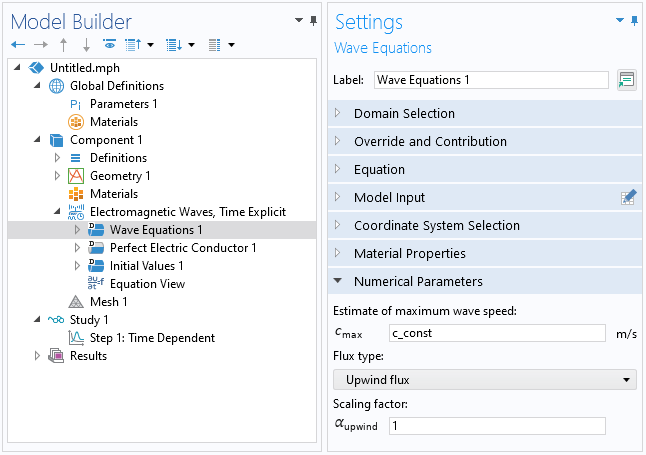
Upwind Flux Formulation

The Flux type parameter in the Wave Equations node for the Electromagnetic Waves, Time Explicit interface now also includes an Upwind flux option. This option can be used to improve S-parameter calculations that may have low accuracy due to overdissipation around perfect electric conductor (PEC) edges, which can occur when using the default Lax-Friedrichs flux parameters.

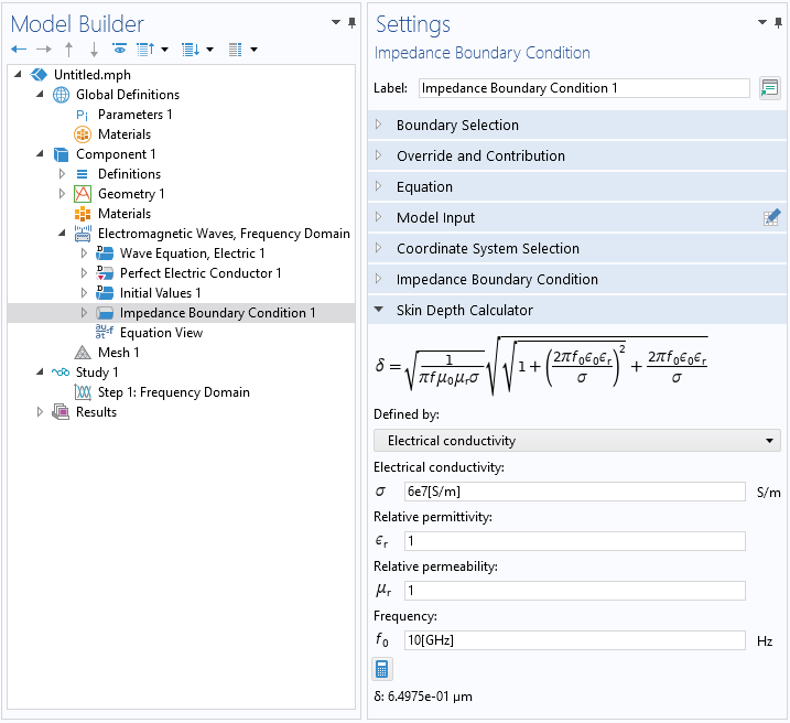
Skin Depth Calculator

A new skin-depth calculator functionality can be used to compute skin depth, which can be defined by the electrical conductivity or resistivity of a material. This can help you determine if the application of a particular boundary condition is appropriate. The Skin Depth Calculator is available in the settings of the Impedance Boundary Condition, Transition Boundary Condition, Layered Impedance Boundary Condition, and Layered Transition Boundary Condition features. The Skin Depth Calculator feature is showcased in the following models:

• beam_splitter
• enhanced_mems_mirror_coating
• graphene_metamaterial_perfect_absorber

New Tutorial Models

COMSOL Multiphysics^® version 6.1 brings several new tutorial models to the Wave Optics Module.

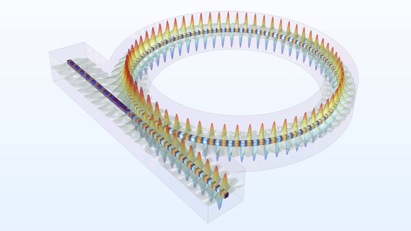
Optical Ring Resonator Notch Filter 3D

A 3D optical ring model using parts from the Wave Optics Part Library. The results show the field distribution at the resonance wavelength.

Application Library Title:
optical_ring_resonator_3D
Download from the Application Gallery

Optical Yagi-Uda Antenna

The Electromagnetic Waves, Boundary Elements interface is used to model an optical Yagi–Uda antenna made of aluminum nanorods. The results show the far-field radiation pattern of the antenna, driven by an electrical point dipole.

Application Library Title:
optical_yagi_uda_antenna
Download from the Application Gallery

Cloaking of a Cylindrical Scatterer with Graphene

The Linearly polarized plane wave background field in a 2D axisymmetric model. The results show a comparison of the field distributions around a cylindrical scatterer with and without a graphene cloak.

Application Library Title:
cylinder_graphene_cloak
Download from the Application Gallery

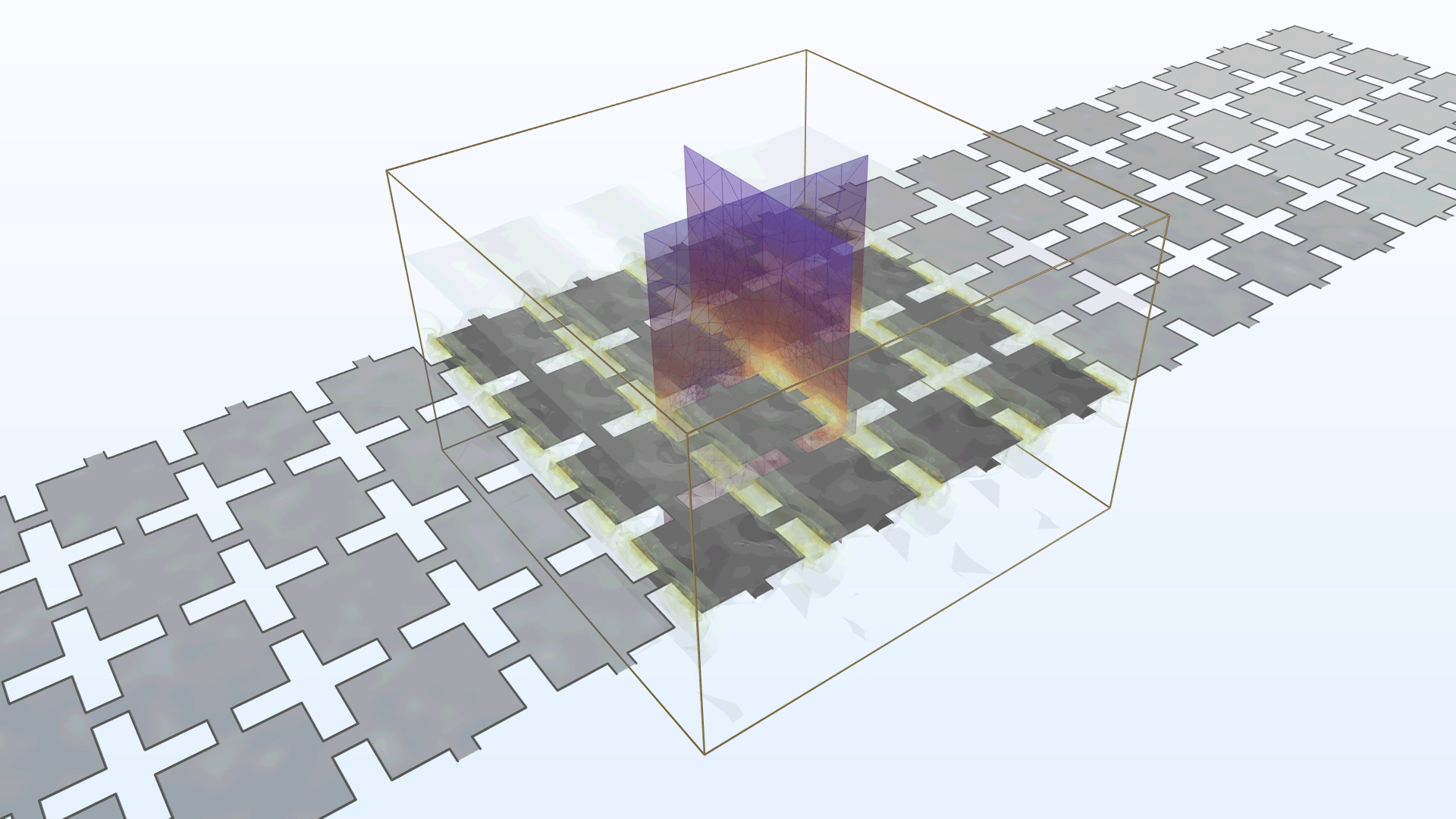
Graphene Metamaterial Perfect Absorber

A graphene-based terahertz (THz) metamaterial absorber, which consists of a fishnet structure.

Application Library Title:
graphene_metamaterial_perfect_absorber
Download from the Application Gallery

Enhanced Coating for a Microelectromechanical Mirror

Comparison of mirror reflectance spectra, before and after optimizing the thickness of the thin dielectric coating layer.

Application Library Title:
enhanced_mems_mirror_coating
Download from the Application Gallery

Tapered Waveguide

The electric field distribution of a tapered waveguide with a propagating wave, modeled using the Electromagnetic Waves, Beam Envelopes interface.

Application Library Title:
tapered_waveguide
Download from the Application Gallery