COMSOL Multiphysics^® 6.1 Release Highlights

Heat Transfer Module Updates

For users of the Heat Transfer Module, COMSOL Multiphysics^® version 6.1 introduces new modeling tools for spacecraft thermal analyses, a multiphysics coupling for defining a continuity condition between shared or facing surfaces, and new tools for defining surface-to-surface radiation models. Read more about the Heat Transfer Module updates below.

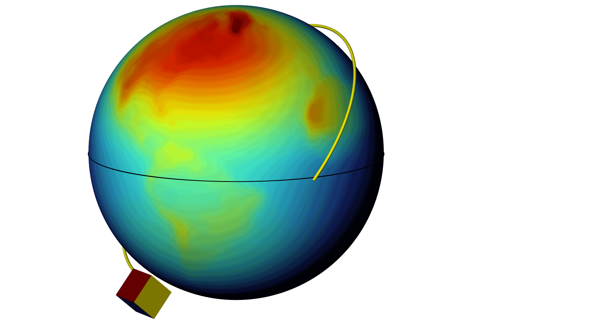
Spacecraft Thermal Analysis

The new Orbital Thermal Loads interface provides ready-made features for modeling radiative loads on a spacecraft, in particular radiation from the Sun and Earth for satellites orbiting around Earth. You can use this feature to include the spacecraft radiative properties, orbit and orientation, orbital maneuvers, and planet properties. The physics interface also computes and generates results that show direct solar radiation, albedo, and planet infrared flux as well as the radiative heat transfer between the different spacecraft parts. When combining this interface with a heat transfer interface, you can account for heat conduction in the solid parts of a spacecraft. You can view this feature in the following new models:

• orbit_calculation
• orbit_thermal_loads
• spacecraft_thermal_analysis

Orbit of a satellite around the Earth. The track color indicates whether the satellite is in eclipse or not. The spacecraft surface color represents the magnitude of the incident solar irradiation. (Earth image credit: Visible Earth and NASA)

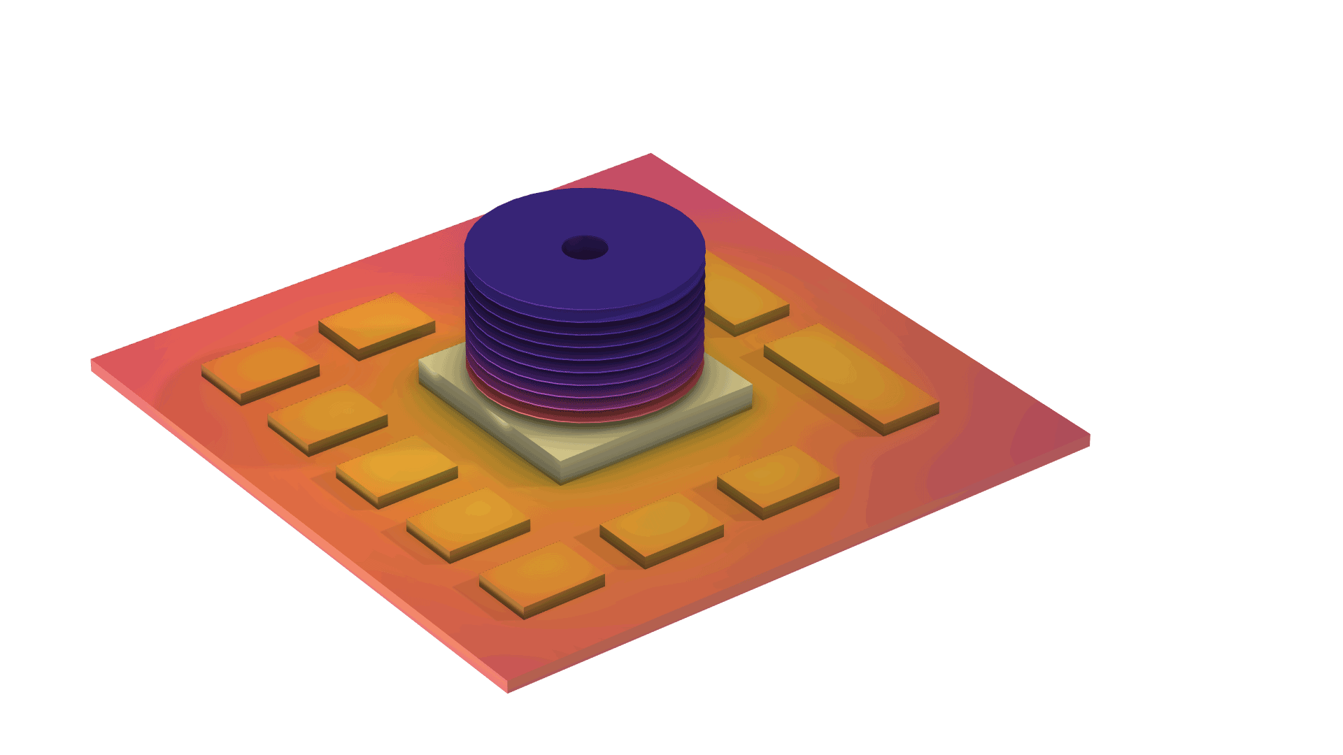
Thermal Connectors Between Shells and Domains

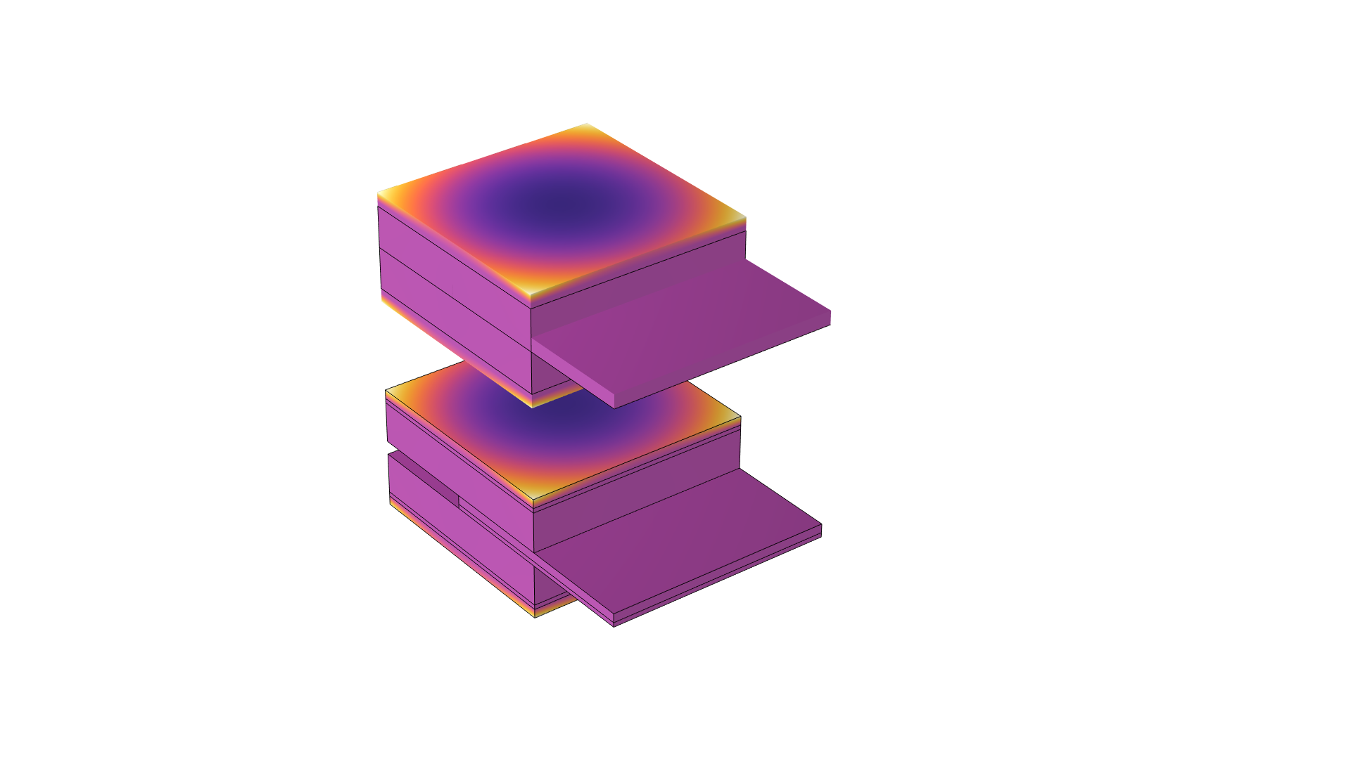
The new Thermal Connection multiphysics couplings are designed to define a continuity condition between two temperature fields, computed by a domain heat transfer interface and a Heat Transfer in Shells interface, respectively. The condition can be set on a boundary shared by the two interfaces or on two boundaries facing each other. The connector can be used for shells that are in contact through an edge, a boundary shared with the domain interface, or a boundary that is facing another boundary from the domain interface. This multiphysics coupling greatly simplifies the use of combined domain and shell interfaces in models. View this feature in the existing Disk-Stack Heat Sink model and the following new tutorial models:

• thermal_connection_by_edges
• thermal_connection_by_facing_boundary
• thermal_connection_by_shared\boundaries

Temperature field in a circuit board (domains) and in a disk-stack heat sink (shell) with a continuity condition set by the Thermal Connector feature.

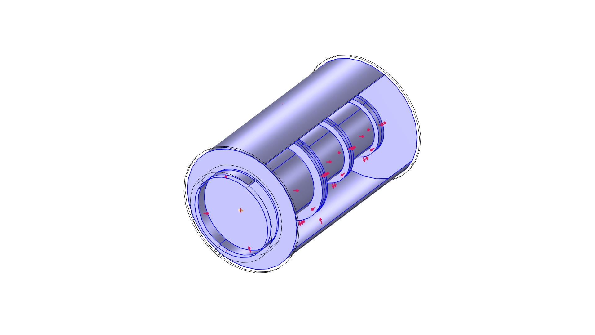
Verification Tools for Surface-to-Surface Radiation Models

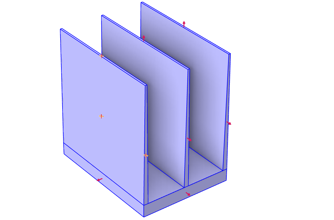
There are new tools available to assist with defining surface-to-surface radiation models. During the model setup, the emitted radiation direction is now represented in the Graphics window with a symbol for the Opacity controlled option and gray surface models. A warning symbol is displayed in the case of unexpected configuration. Furthermore, during the view factor evaluation, an optional verification is available to detect inconsistent topology. These tools greatly reduce the risk of erroneous definition of models, especially for large and complex geometrical configurations. View these updates in the new Topology Verification for Surface-to-Surface Radiation model and these existing models:

• cavity_radiation
• chip_cooling
• heat_sink_surface_radiation
• inline_induction_heater
• light_bulb
• parallel_plates_diffuse_specular_ray_shooting
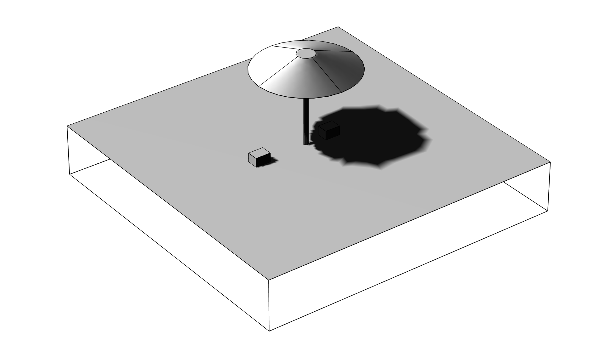
• parasol
• potcore_inductor
• thermal_annealing
• tpv_cell
• view_factor
• petzval_lens_stop_analysis_with_surface_-_to_-_surface_radiation

Model geometry with arrows representing the emitted radiation direction. The exclamation mark (front, center) indicates a boundary where no radiation direction is defined.

Surface-to-Surface Radiation Improvements

The ray-shooting method has been improved so that small surfaces are detected even when a coarse resolution is used for the view factor evaluation. Combined with the resolution adaptation, this improves the view factor accuracy with an optimal number of rays. In addition, for all view factor computation methods, expressions used to define variables and equations are now preprocessed so that their readability is facilitated and their evaluation is much faster during the assembly step. The following models showcase these new improvements:

• cavity_radiation
• chip_cooling
• heat_sink_surface_radiation
• inline_induction_heater
• light_bulb
• parallel_plates_diffuse_specular_ray_shooting
• parasol
• potcore_inductor
• thermal_annealing
• tpv_cell
• view_factor
• petzval_lens_stop_analysis_with_surface_-_to_-_surface_radiation

This model shows solar heat flux at the beach, where two styrofoam coolers contain beverage cans. A parasol provides shade for one of the coolers, and the temperature of the beverage cans is computed over time.

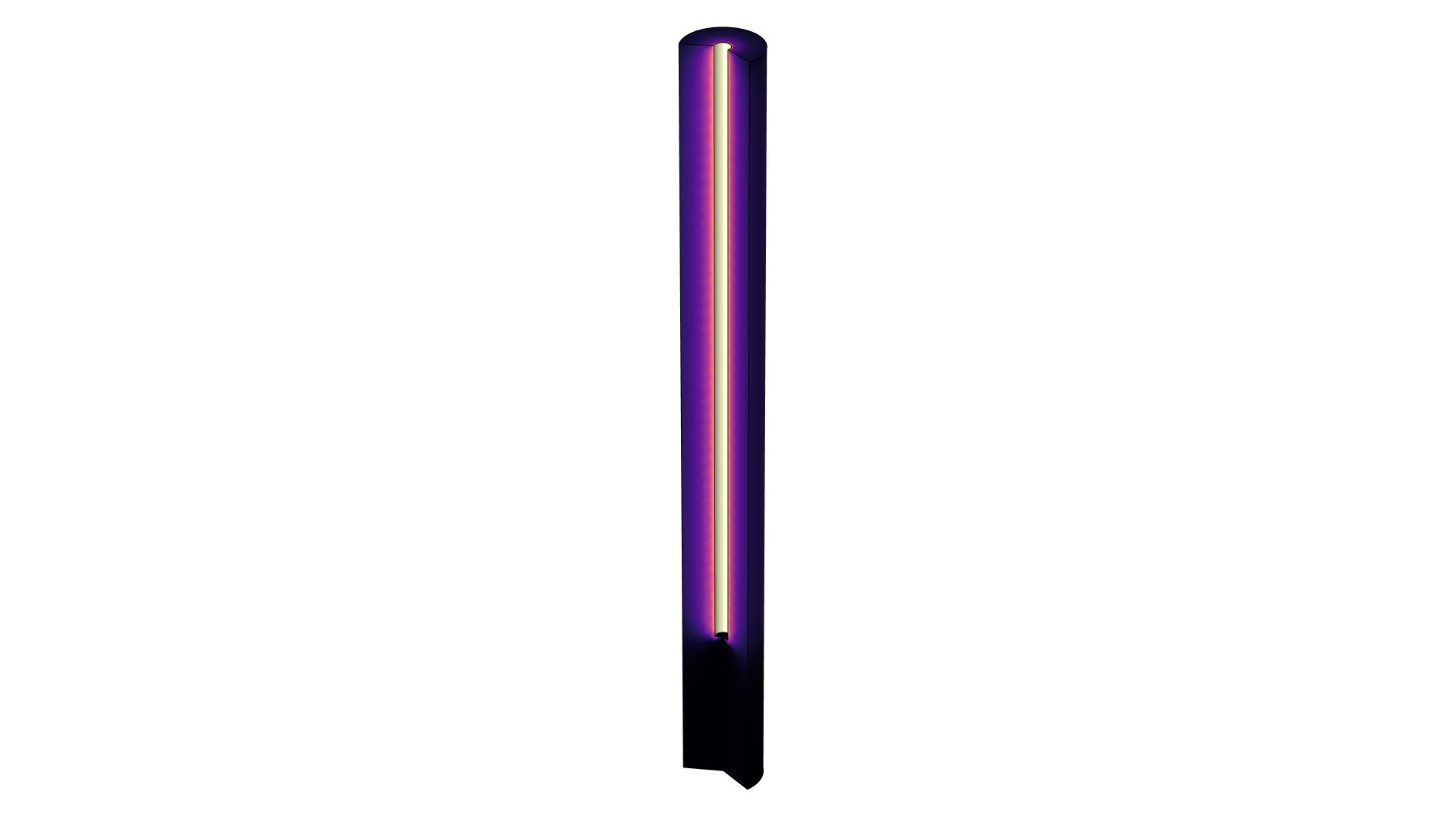
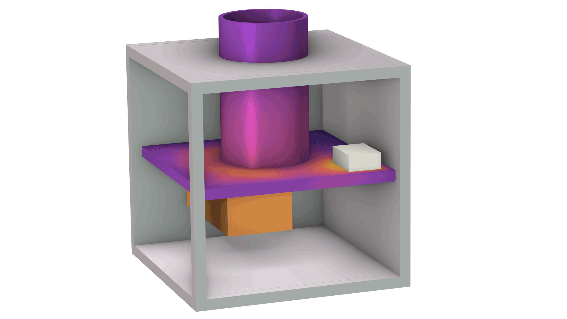
Fluence Rate

In the Surface-to-Surface Radiation interface, it is now possible to add a Fluence Rate Calculation node in order to select the domains where the fluence rate has to be computed. The fluence rate indicates the exposure to radiation if a small object is placed in a cavity. This is useful when you want to, for example, check the UV exposure in a water purification reactor. You can view this new feature in the Annular Ultraviolet Reactor, Transparent Water model.

Fluence rate in an ultraviolet reactor filled with quasitransparent water.

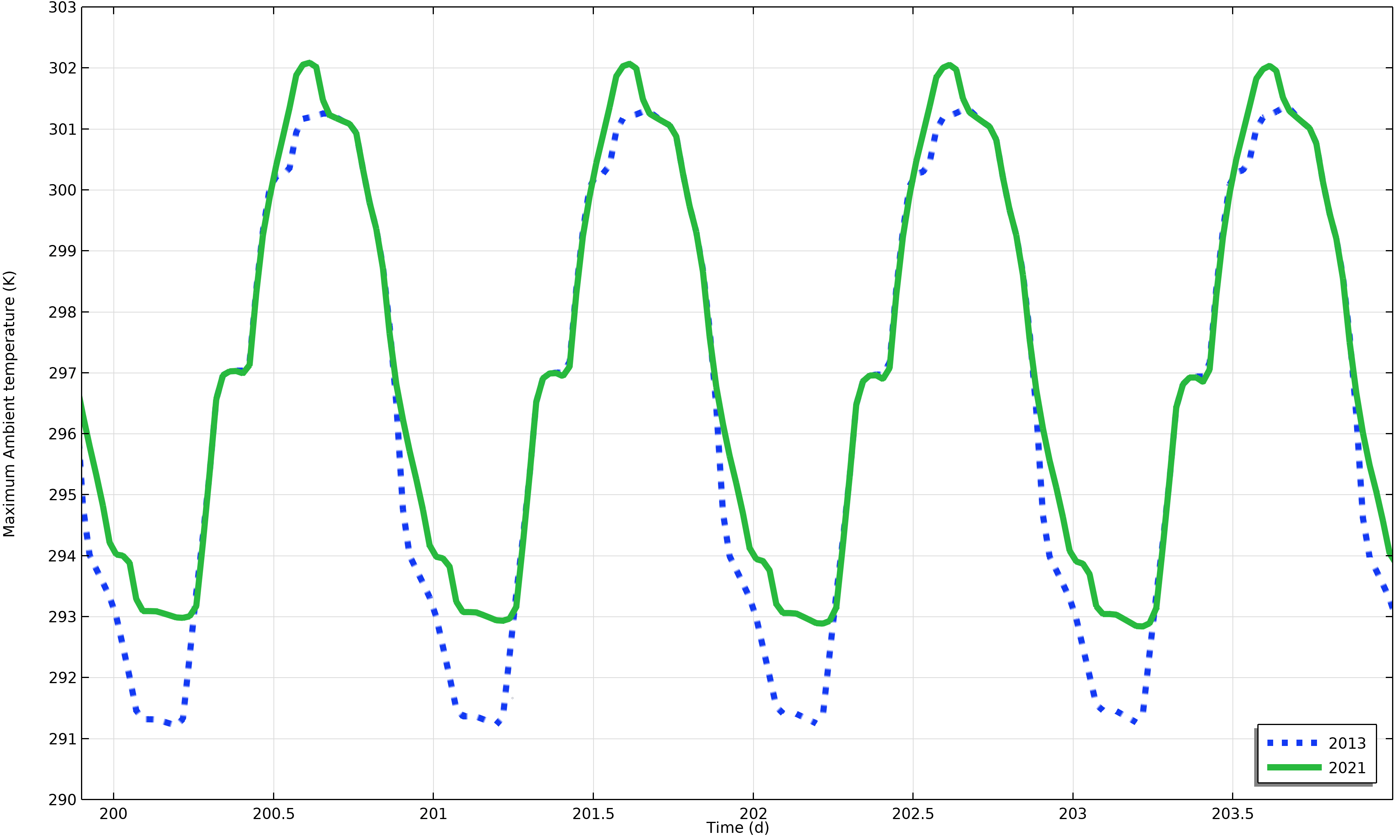
Climate Data: ASHRAE 2021

Ambient properties, such as temperature, humidity, precipitation, and solar radiation, can be defined from an Ambient Properties node under Definitions > Shared Properties. Along with the possibility of adding user-defined meteorological data, ambient variables can be computed from monthly and hourly averaged measurements from values in handbooks provided by the American Society of Heating, Refrigerating, and Air-Conditioning Engineers (ASHRAE). The meteorological data from the ASHRAE 2021 handbook has been integrated into COMSOL Multiphysics^® and contains ambient data from more than 8500 weather stations around the world.

You can view this new feature in the following existing models:

• condensation_electronic_device
• isothermal_box
• wood_wall_frame

Maximum temperatures on the hottest days of the year (blue, 2013; green, 2021) at a weather station in Glasgow, UK, show that measured temperature increased after 2013. Data from ASHRAE Weather Data.

Enhanced Thermal Wall Functions for Viscous Dissipation

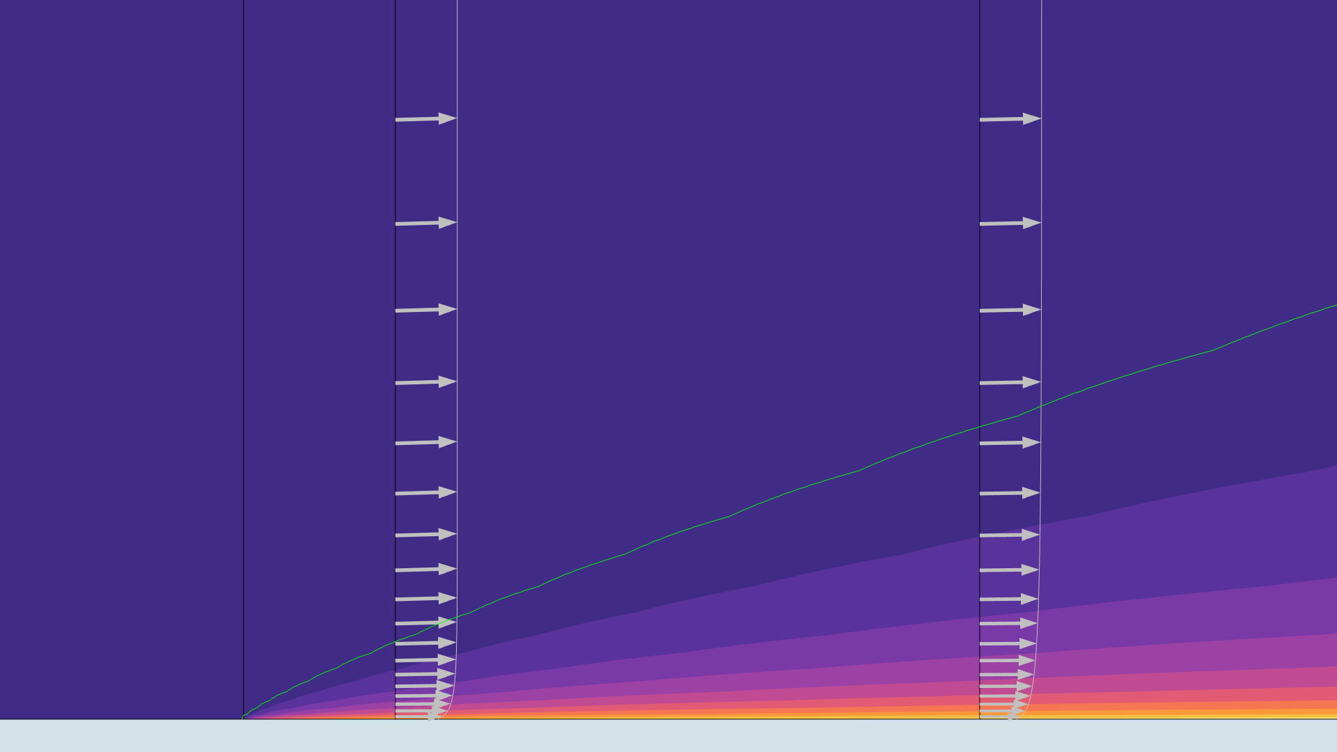
In the Nonisothermal Flow coupling under its Heat Transfer Turbulence settings, a new Thermal wall function setting is available for Reynolds-averaged Navier–Stokes (RANS) turbulence models. There are two options available: Standard, which is suitable for most configurations, and High viscous dissipation at wall, which accounts for viscous dissipation in the boundary layer. This is needed for accurate results in the case of fast internal flow, especially for narrow paths or if the fluid is very viscous. The new Zero Pressure Gradient 2D Flat Plate model highlights this new feature.

Temperature profile (surface plot) induced by viscous dissipation close to the wall and velocity direction (arrows). The green curve indicates the limit of the boundary layer (99% U_inf), and the cyan curves indicate the velocity profile at x = 0.97 m and x = 1.9 m.

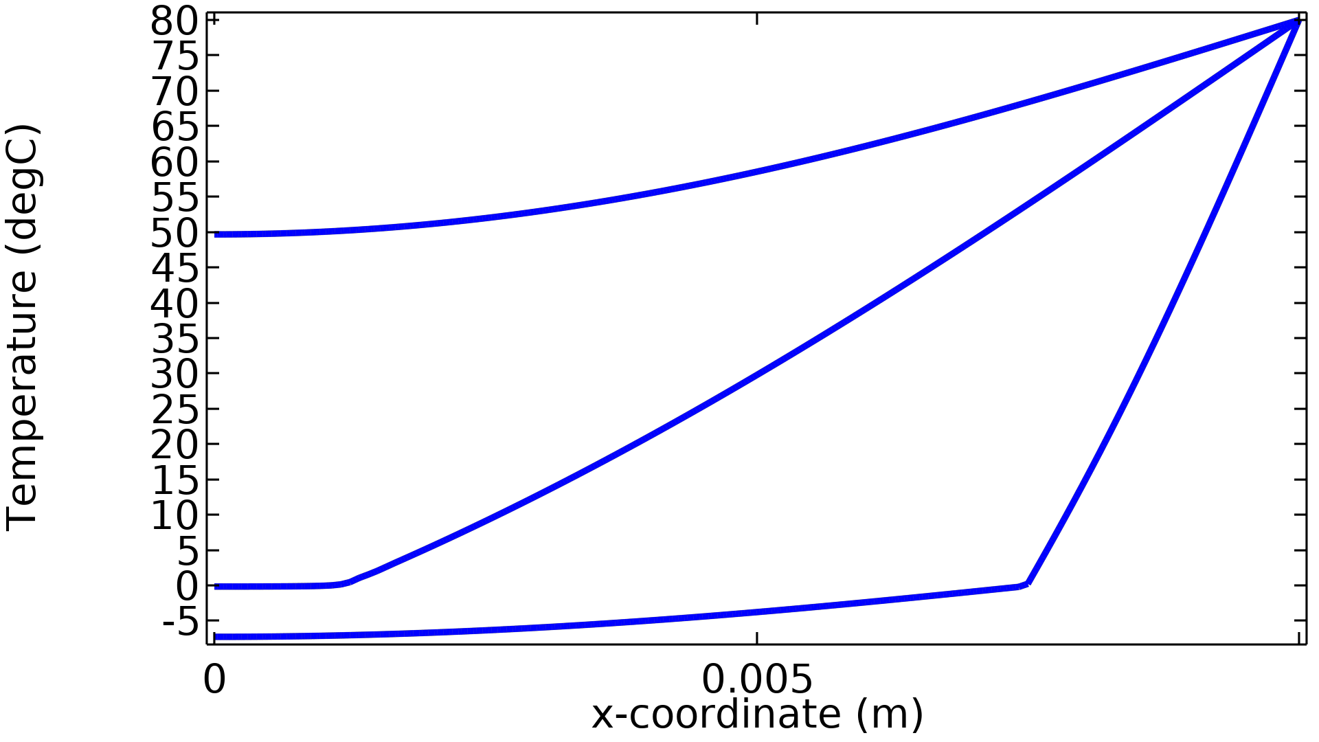
User-Defined Phase Transition Function for Phase Change Material

In the Phase Change Material feature, a User-defined phase transition function is available that enables more accurate description of material properties. This option makes it possible to use accurate phase change descriptions from measured or material databases. View this update in the new Phase Change in a Semi-Infinite Soil Column - Lunardini Solution model and the following existing models:

• continuous_casting_apparent_heat_capacity
• cooling_solidification_metal
• frozen_inclusion
• isothermal_box
• phase_change

Temperature profile in an initially frozen domain heated over time.

Additional Features for Moisture Transport in Hygroscopic Porous Media

To simplify model definitions, the Moisture Flow multiphysics coupling has been updated so that the evaporation rate variable computed by the Moisture Transport interface is accounted for in the mass balance computed by the Brinkman Equations interface. In addition, the Open Boundary and Inflow boundary conditions can now be applied to exterior boundaries adjacent to domains where the Hygroscopic Porous Medium is active.

New Tutorial Models

COMSOL Multiphysics^® 6.1 brings several new tutorial models to the Heat Transfer Module.

Orbit Calculation

Orbit and incident irradiation of a 1U CubeSat at 400 km altitude, with an inclination of 50° and the longitude of the ascending node at 0°. The black color of the orbit track indicates the eclipse. The total irradiation and the radiative loads from all environmental sources are computed.

Application Library Title:
orbit_calculation
Download from the Application Gallery

Orbit Thermal Loads

Spacecraft orbit and incident irradiation. The color on the Earth surface represents the albedo magnitude. A satellite in orbit experiences solar, albedo, and planetary infrared (IR) loads, where albedo and planetary IR can vary with latitude and also with longitude. The total irradiation and flux on the satellite are evaluated over several orbits.

Application Library Title:
orbit_thermal_ loads
Download from the Application Gallery

Spacecraft Thermal Analysis

Temperature distribution in a satellite circuit board with electrical components. The direct solar, albedo, and Earth IR thermal loads are precomputed in an Orbit Thermal Loads study and reused on multiple orbit periods in an Orbital Temperature study.

Application Library Title:
spacecraft_thermal_analysis
Download from the Application Gallery

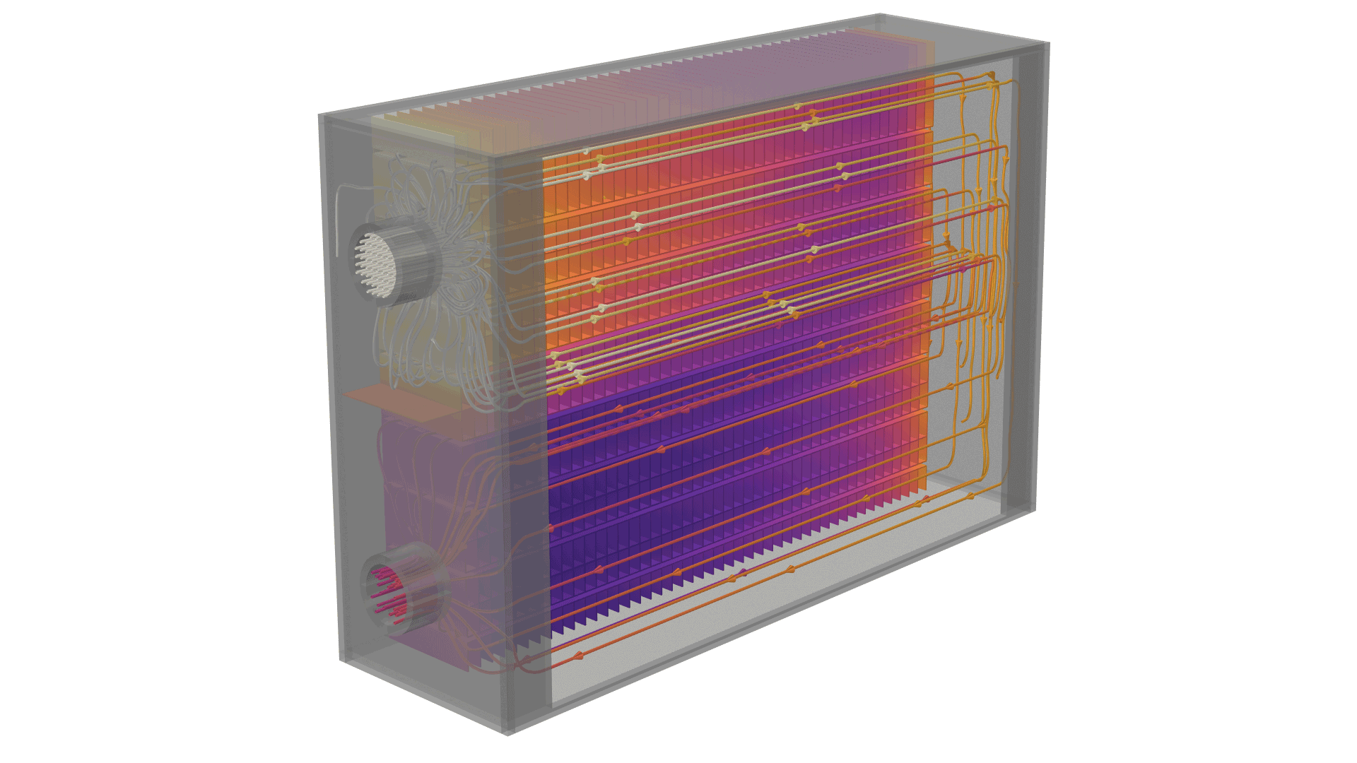
Plate-Fin Heat Exchanger

Oil flow and fins temperature in a plate-fin heat exchanger. In order to maximize heat transfer, the heat exchanger is made of a porous aluminum matrix in which the hot oil flows. Heat is conducted through aluminum fins in contact with the porous matrix. These fins are modeled as thin layers, meaning their thickness is not drawn in the geometry but is taken into account in the heat transfer model.

Application Library Title:
plate_fin_heat_exchanger
Download from the Application Gallery

Zero Pressure Gradient 2D Flat Plate

The temperature profile (surface plot) and velocity direction (arrows) of the Zero Pressure Gradient 2D Flat Plate model. The plot shows the behavior of a turbulence model and wall functions in the boundary layer of a turbulent flow.

Application Library Title:
zero_pressure_gradient_2d_flat_plate
Download from the Application Gallery

Annular Ultraviolet Reactor, Optically Transparent Water

Fluence rate in an ultraviolet reactor filled with quasitransparent water. The reactor contains an annular fluid region surrounding a cylindrical lamp.

Application Library Title:
annular_ultraviolet_reactor_optically_transparent_water
Download from the Application Gallery

Thermal Connector Tutorial Models

Comparison of the temperature field in two similar structures. The bottom structure is computed in a classical geometry made of different domains. The top structure is computed as a combination of domains and shells that are connected using the Thermal Connector coupling.

Application Library Titles:
thermal_connection_edges
Download from the Application Gallery
thermal_connection_facing_boundary
Download from the Application Gallery
thermal_connection_shared_boundaries
Download from the Application Gallery

Topology Verification for Surface-to-Surface Radiation

Automatic detection of suspicious radiation-direction definition in the user interface. The warning symbols indicate the boundaries where inconsistent radiation settings have been identified.

Application Library Title:
topology_verification_nonradiating
Download from the Application Gallery