support@comsol.com
COMSOL Desktop® Updates
For all COMSOL Multiphysics® users, version 6.1 introduces the ability to create and edit parameters directly from edit fields, a new Find and Replace tool, and table usability improvements. Read more about these updates below.
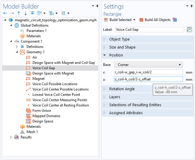
Create and Edit Parameters in Model Settings
A new streamlined workflow enables you to create parameters without the need to navigate to a Parameters node. Within text fields and tables in the Settings window, you can now right-click to select the Create Parameter feature to specify the name, expression, and description of the new parameter. Similarly, if you right-click in a text field or table cell with a parameter in an expression, you can choose the Edit Parameter option to edit the parameter's Name, Expression, and Description fields.
The Create Parameter option is used to specify a parameter for the electric potential. Creating the parameter replaces the input field content (or the selected part, if any) with the parameter name. The Edit Parameter option is used to modify the thickness of the busbar.
In addition to manipulating parameters, it is now easier to see the value of parameter expressions. When you hover over input fields and table cells, a tooltip shows the assessed value of the expression.
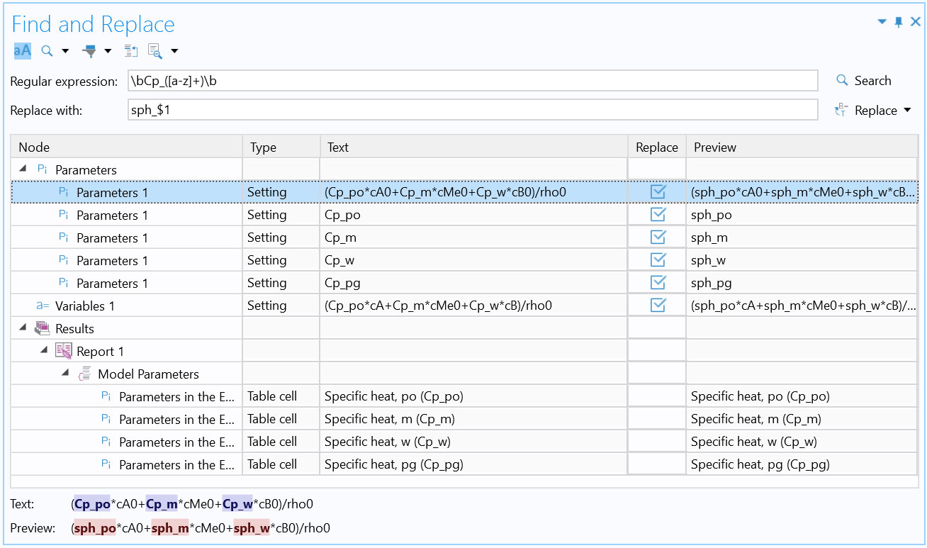
Find and Replace
The new Find and Replace tool comes with a Replace functionality to replace any matches that come up in your search. Search results have a structured hierarchy, so you can easily hide parts that are not relevant to a specific search. You can also narrow your search by using Nodes, Descriptions, and Settings filer options to limit what is shown in the search results. There is also a Search History menu that lists your previous searches and enables you to perform them again.
Table Usability Improvements
When loading parameters in older versions, if there were already existing parameters, you would get duplicate entries, which you had to manually remove. In this version, when loading from text and CSV files, you can now directly update existing parameters or variables in tables. Any new parameters in the file are added as usual.
When loading from external files, you now have the option to update existing values.
You can now directly insert a row above any selected row in a table. In previous versions, tables only allowed you to add a row at the bottom and then move it into place.
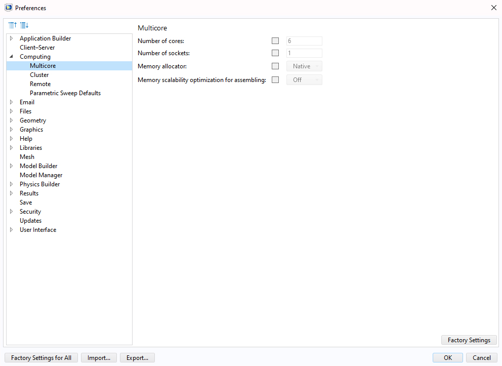
New Categorization of Preferences
The Preferences dialog box now contains a tree of categories instead of a list, making it easier to locate related preferences.
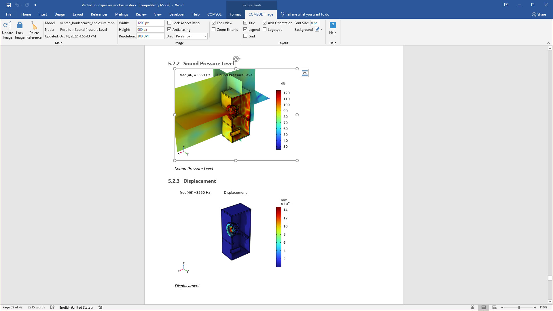
Interface for Microsoft® Word
A new COMSOL ribbon tab in Microsoft® Word is available for inserting and updating images and tables from COMSOL models. Within the COMSOL® software, images and tables can be generated for the clipboard, which enables them to remain linked to the COMSOL model file when inserted into a Microsoft Word document. The report generator now saves linked images and tables when saving a report to the Microsoft Word format. Then, in Microsoft® Word, you can update linked images and tables to reflect changes in the solution, for example.
Miscellaneous Additions
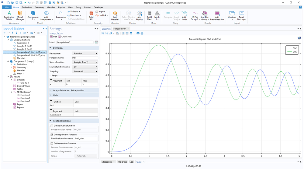
Primitive and Inverse Functions
You can now define primitive functions of user-defined functions. This functionality is available as a generalization of existing functionality for generating primitive functions for interpolation functions. The new functionality is available in the settings for the Interpolation function feature, in which you reference an arbitrary user-defined function for which the primitive function should be defined. Primitive functions are also known as antiderivatives or indefinite integrals. In a similar way, you can define inverse functions of user-defined functions.
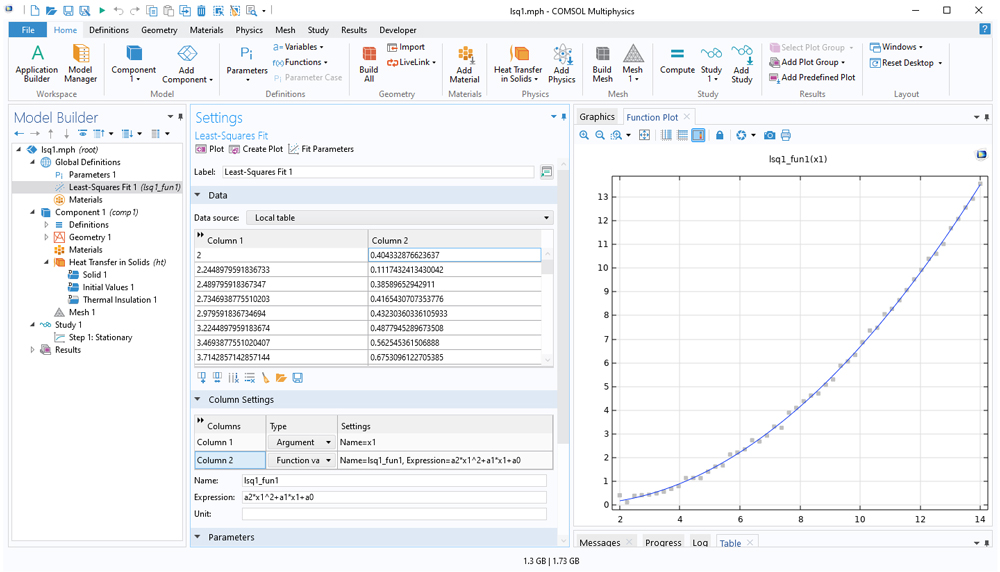
Least-Squares Fit Function
A new Least-Squares Fit function allows for the fitting of tabulated multidimensional function data to one or more arbitrary parametric function expressions. This functionality was previously exclusive to the Optimization Module, in which it was used for linear regression as well as the fitting of parametric nonlinear functions. You can now define Least-Squares Fit functions directly under the Definitions node in the Model Builder. For example, you can fit a function such as (a0+a1*x+a2*y)*cos(a4*z+a5) with respect to three-dimensional input data. The Least-Squares Fit function requires one of the following products: the Battery Design Module, Optimization Module, or Polymer Flow Module. However, in a future software update, this functionality will be made available without requiring any add-on product.
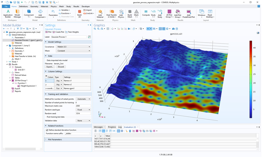
Gaussian Process Function
A new Gaussian Process function allows for multidimensional interpolation of data together with estimates of the uncertainty in the interpolated function. The Uncertainty Quantification Module is required for training the function with respect to input tabulated data. However, if a function is already trained and is stored in a model, it does not require any add-on products.
Spatial Derivates for Coupling Operators
Both the spatial at operator and nonlocal coupling operators, such as General Extrusion, now include the contributions from mapping to the spatial derivatives. This enables a wider range of field mappings. For example, you will now be able to directly map an acoustic pressure field or electromagnetic field from one component to another without intermediate steps.
Faster Evaluation of Expressions Using Solution Parameters
The new withparam operator is a specialized version of the previously available withsol operator that evaluates faster than withsol when applicable, such as when solving study steps in a sequence. A typical example when withparam can be used is when solving for electromagnetic heating in a sequence of two steps, where the first step is solving for electromagnetic fields in the frequency domain and the second step is solving for heat transfer using a frequency-dependent source term with frequency values from the first step. More generally, withparam is useful for sequential solving when time (t), frequency (freq), or eigenvalue (lambda) variables from a previous study step are used in a subsequent study step.
New Built-In Functions
Two new built-in functions are available for computing the greatest common divisor (gcd) and least common multiplier (lcm). These functions have a wide range of applications, including when analyzing symmetries of electric motors and generators.