Technical Papers and Presentations

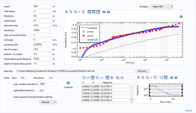
In a pumping test the drawdown of the water table in a piezometer is recorded, as response to pumping from a nearby well. Pumping tests belong into the common toolbox of hydro-geologists, used to obtain basic parameters for aquifer characterization. There are various approaches to evaluate the recordings from pumping tests. It is common practice to determine transmissivity (T) and storativity (S) from fitting 1D-analytical solutions to the observed drawdown. However, often situations are dealt with in which the simple 1D-approach is not justified. These cases can be handled by numerical methods. We present an app tool, built by the COMSOL® Application Builder that handles general 2D flow. The created graphical user interface (GUI) is shown in the figure.

The application is based on a 2D model for a vertical cross-section, which represents the aquifer from the borehole wall to the reach of the well. The following geometric properties that can be considered: the thickness of the aquifer, the location of the well screen and the depth position of the observation point. These parameters are often known, but the common evaluation practice doesn’t take advantage of this knowledge.

The parameter estimation is performed using the COMSOL® Optimization Module. While T and S parameters are determined by default, other unknown parameters can be included in the estimation procedure, such as the reach of the well, the thickness of the aquifer, initial position of the water table, groundwater recharge and the ratio of hydraulic conductivities. The model was verified using data performed for tests in confined aquifers, which were also handled by the common 1D approach. Moreover, in most applications it was possible to improve the fit in comparison to the 1D evaluation. It is intended to extend the current model to deal with pumping tests in unconfined and leaky aquifers.The figure shows the Pump Test App, developed using the COMSOL® Application Builder. The input parameters and their values are listed on the left of the panel. Below one finds the button to browse the file with the input data recorded during pumping. The ‘Compute’ button below initiates the model run. In the left bottom corner some options of the optimization solver can be specified. The model output is shown in the center graph, depicting measurements and model output for the optimized parameter set. The parameter values are listed in the table below. The plot on the lower right visualizes the advancement of the objective function during the optimization process.

In conclusion, 2D numerical methods can be used successfully for the evaluation of pumping tests. They are superior to methods based on 1D analytical solutions, as they are built on less restrictive assumptions. Moreover, one can take advantage of a better site characterization by including known parameters in the model.