Mode Superposition
What Is Mode Superposition?
When performing dynamic response analyses of linear structures, mode superposition is a powerful technique for reducing the computation time. Using this method, the dynamic response of a structure can be approximated by a superposition of a small number of its eigenmodes.
Mode superposition is most useful when the frequency content of the loading is limited. It is particularly useful when performing analyses in the frequency domain, since the loading frequencies are known. Wave propagation problems are not suited for this technique, as they involve very high frequencies.
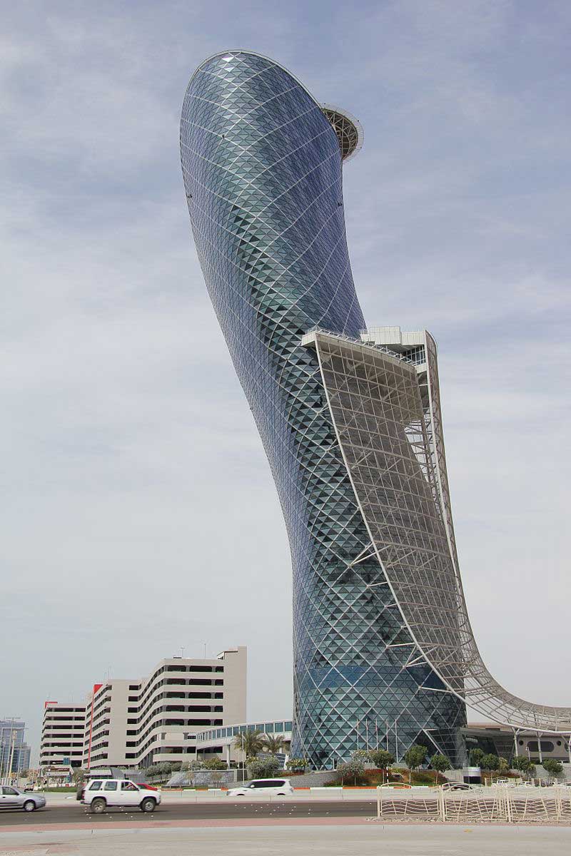
Mode superposition is a common tool in seismic engineering, since the frequency content in earthquakes is limited. Image by FritzDaCat — Own work. Licensed under CC BY-SA 3.0, via Wikimedia Commons.
Mode superposition is a common tool in seismic engineering, since the frequency content in earthquakes is limited. Image by FritzDaCat — Own work. Licensed under CC BY-SA 3.0, via Wikimedia Commons.
Deriving the Modal Equations
Assume that the equations of motion for a structure are written in matrix form as

where  is the mass matrix,
  is the damping matrix, and
  is the stiffness matrix. The degrees of freedom (DOFs) are placed in the column vector
  and the forces in
  .
.
Often, the matrix form is obtained from a discretization of a physical problem using the finite element method. If N denotes the number of DOFs, the matrices have the size NxN.
Here, it is assumed that the matrices are real and symmetric and that the stiffness matrix is positive definite. This is the most common case, but it is also possible to use mode superposition in the case of unsymmetric matrices. This could happen, for example, in a coupled acoustic-structural problem. The theory when using unsymmetric matrices is somewhat more complicated, but the principles are the same.
A prerequisite for a mode superposition is to compute eigenfrequencies and corresponding mode shapes. This is usually done for the undamped problem, using the eigenvalue equation

Usually, only a small number n of the eigenfrequencies are computed. The result of this computation is a set of natural frequencies  with corresponding mode shapes
  , where i ranges from 1 to n. It can be shown that the eigenmodes are orthogonal (or, in the case of duplicate eigenvalues, can be chosen as orthogonal) with respect to both the mass and stiffness matrices. This means that

and

It is convenient to place the eigenmodes in a rectangular Nxn matrix  , where each column contains an eigenmode. The orthogonality relation can then be summarized as

The diagonal elements are called the modal masses. The values of the modal masses depend on the chosen normalization of the eigenmodes. This normalization is arbitrary, since the mode only represents a shape and the amplitude does not have a physical meaning. One common and convenient choice is mass matrix normalization. The eigenmodes are then scaled so that each  , giving

The corresponding orthogonality relation for the stiffness matrix is

If mass matrix normalization is used, the diagonal matrix  consists of the squared natural angular frequencies.
The basic assumption in mode superposition is that the displacement can be written as a linear combination of the eigenmodes:

Here,  are the modal amplitudes.
If all eigenmodes of the system were used, this would be an exact, rather than approximate, relation. Since the eigenmodes are orthogonal, they form a complete basis and the expression is merely a change of coordinates from the physical nodal variables to the modal amplitudes. When only a small number of eigenmodes are used, the mode superposition can be viewed as a projection of the displacements onto the subspace spanned by the chosen eigenmodes.
The mode superposition can also be written in matrix form as

where the modal DOFs have been collected in the column vector  .
.
Inserting the mode superposition expression in the equation of motion gives

After a left multiplication by  :
:

It will be possible to make use of the orthogonality relations so that

The original system of equations has now been reduced from N to n variables. The right-hand side  is called the modal load. Solving this smaller problem will significantly reduce the computational effort, but there is one more possible simplification. Since
  and are diagonal matrices, only the
  term provides a coupling between the equations. It is commonly assumed that the modal damping matrix is diagonal, so that a set of uncoupled equations of the type

can be used.
However, it should be noted that in real life, there is often some crosstalk between different vibration modes in a damped structure. If strong physical damping is present, like when discrete dashpots are used, it is preferable to use the coupled system.
Damping Models
Damping models that can provide decoupled equations in mode superposition include:
- Modal damping
- Rayleigh damping
- Caughey series
- Lumping
Modal Damping
Directly providing the damping ratio for each mode,  , is a common choice. Modal damping gives a large degree of control. Modes can be assigned a higher damping value if, for physical reasons, they are expected to be strongly damped.
Rayleigh Damping
In the Rayleigh damping model, the damping matrix is assumed to be a linear combination of the mass and stiffness matrices,

where  and
and  are the two parameters of this model.
It will thus be diagonalized by the eigenmodes, just like the constituent matrices. The modal damping will thus be defined implicitly as

The coefficients and are usually chosen so that the damping is reasonable at two different frequencies in the interval of interest.
The merit of the Rayleigh damping model is its simplicity; it does not have any physical significance.
Caughey Series
There are actually more general expressions where the damping matrix can be diagonalized by the eigenmodes. A damping matrix constructed using a Caughey series

has the same orthogonality properties. The modal damping will be

Rayleigh damping is the special case of using the first two terms of the Caughey series. In practice, a Caughey series approach is seldom used.
Lumping
One possible way to create a diagonal modal damping matrix is to use some kind of lumping scheme on to create a diagonal matrix. The simplest such scheme would be to just drop all off-diagonal elements.
The Modal Load
The modal load  is a projection of the external load onto each of the eigenmodes. If a load has a very small projection on a certain mode, such a mode does not need to be included in the superposition. A common case is when both the structure and the load are symmetric. All antisymmetric eigenmodes can then be ignored, since there is no projection of the load on these modes.
Since only a small subset of the modes is used in the response analysis, some fraction of the total original load is lost during the projection to the modal coordinates. Various schemes for improving the solution are available; for example, static correction, mode acceleration, and modal truncation augmentation.
Stresses and Strains
In general, to obtain good stress results, more modes must be used in the superposition than what are needed for a good representation of the displacements. This is because higher modes generally have more complex mode shapes. The derivatives of the displacements (that is, the strains) are thus relatively higher. Examining modal stresses for the individual eigenmodes can indicate their relative importance.
Moving Foundations
All eigenmodes will have zero displacements in DOF where the displacements are constrained. Thus, it is not straightforward to model an excitation by a moving foundation using mode superposition, since such a displacement is not contained in the base spanned by the mode shapes.
However, a common case is that the whole foundation moves synchronously, such as a building subjected to an earthquake. The analysis can be performed in a coordinate system fixed to the foundation. This implies that the acceleration of the foundation is instead transformed into volume forces.
There is also a technique that is commonly referred to as the large mass method. In this approximate method, each nonzero-prescribed displacement is replaced by a very large point mass. This will give rise to a few very low eigenfrequencies in which only the masses are moving, but all other eigenfrequencies and modes will be almost unchanged. In effect, this means that the set of shapes available in the superposition has been augmented by something rather similar to the static solutions to unit-prescribed displacements.
Mode Superposition of a Simply Supported Beam
Consider a simply supported beam with the following properties:
- Young's modulus, E = 210 GPa
- Mass density, ρ = 7850 kg/m3
- Area moment of inertia, I = 7960 mm4
- Cross-section area, A = 1000 mm2
- Length, L = 12 m
 A simply supported beam.
A simply supported beam.
A simply supported beam.
The natural frequencies for a simply supported beam are given by the expression

which, with the selected values, evaluates to  .
.
The corresponding eigenmodes can be shown to be

where  are the arbitrary normalizing constants.
We consider the continuous analytical solution in which the equivalent to the mass matrix normalization is

For all modes,

Let us consider a distributed load with constant intensity  per unit length.
The modal load can be computed as

For even values of j, the modal load is zero. This reflects the fact that the load is symmetric, while the even-numbered modes are unsymmetric. For odd values of j, the modal load is

In order to compute a specific response, let us assume that the line load is harmonic with

With the angular frequency of 22 rad/s being close to the natural frequency of the 5th eigenmode, we can expect the mode to have a significant influence on the total response. Without any damping and with mass normalization, the modal equations are

With a harmonic excitation with amplitude  , we obtain the frequency domain version,

The modal amplitude can be explicitly solved for. The result is

It is thus possible to write the displacement based on the mode superposition explicitly as

Taking the second derivative gives the bending moment, so that

Except for changed constant multipliers, it can be noted that the term 2k + 1 has moved from the denominator to the numerator. This means that the higher modes are influencing the bending moment (thus the stresses) more than the displacements.
In the table below, the modal loads and modal amplitudes are computed for the first ten eigenmodes for the value  .
.
| Mode j | ωj | rj | qj |
|---|---|---|---|
| 1 | 1 | 11.13 | -2.30·10-2 |
| 2 | 4 | 0 | 0 |
| 3 | 9 | 3.71 | -9.21·10-3 |
| 4 | 16 | 0 | 0 |
| 5 | 25 | 2.23 | 1.58·10-2 |
| 6 | 36 | 0 | 0 |
| 7 | 49 | 1.59 | 8.29·10-4 |
| 8 | 64 | 0 | 0 |
| 9 | 81 | 1.24 | 2.03·10-4 |
| 10 | 100 | 0 | 0 |
The modal amplitudes decrease in higher modes ( ), since
  .
.
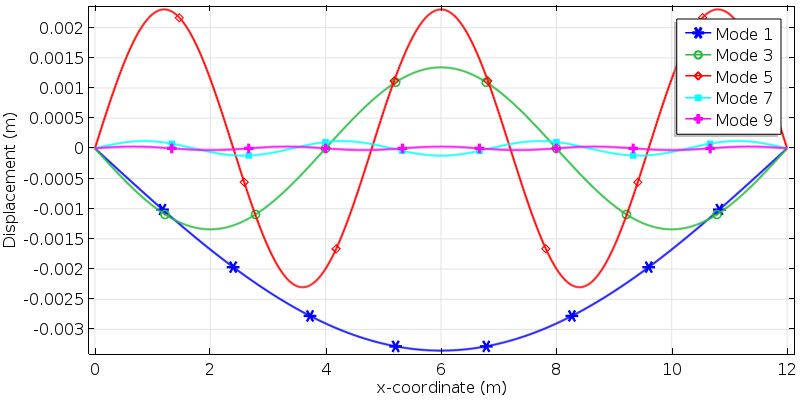 Contributions to the displacement from the first ten modes.
Contributions to the displacement from the first ten modes.
Contributions to the displacement from the first ten modes.
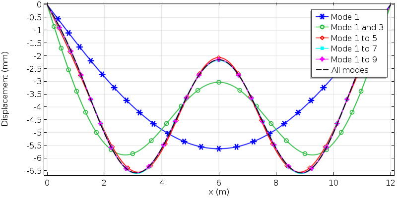
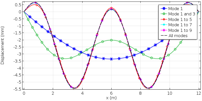 The displacement along the beam after successive summation of the modes.
The displacement along the beam after successive summation of the modes.
The displacement along the beam after successive summation of the modes.
The displacement results are already well converged when summing modes 1, 3, and 5. In order to get a good representation of the bending moment, mode 7 must, at least, also be included.
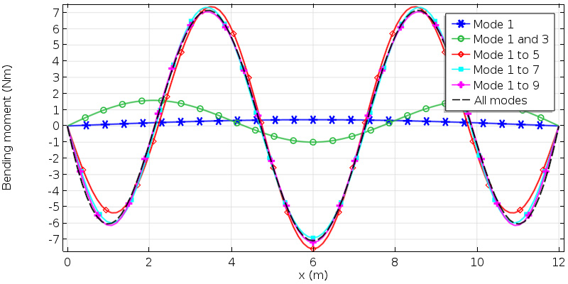 The bending moment along the beam after successive summation of the modes.
The bending moment along the beam after successive summation of the modes.
The bending moment along the beam after successive summation of the modes.
In this example, the response is strongly dominated by a single mode: mode 5. If the forcing angular frequency is shifted from 22 rad/s to 17 rad/s, we move away from the resonance. The results are shown in the following figures.
The displacement is now dominated by mode 3, even though the inclusion of mode 5 is necessary to get an acceptable solution. The bending moment, however, is still dominated by mode 5.
 The displacement along the beam after decreasing the forcing frequency.
The displacement along the beam after decreasing the forcing frequency.
The displacement along the beam after decreasing the forcing frequency.
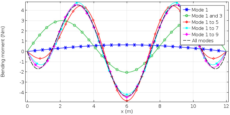 A bending moment along the beam after decreasing the forcing frequency.
A bending moment along the beam after decreasing the forcing frequency.
A bending moment along the beam after decreasing the forcing frequency.
Last modified: May 8, 2018