

The year is 1985, and the world’s focus on space exploration is in full swing. The Salyut 7, a Soviet space station, orbits Earth, but something is wrong. Russian scientists cannot get in contact with Salyut 7. All systems are shut down, and the craft is beginning to drift out of its orbit…
Discovering the Dzhanibekov Effect
Cosmonauts Vladimir Dzhanibekov and Viktor Savinykh were sent to save the spacecraft. It was a difficult mission. According to award-winning historian and science writer David S. F. Portree, it was “one of the most impressive feats of in-space repairs in history.”
Supplies from Earth were locked down with wingnuts, which have three axes of rotation. As Dzhanibekov unscrewed the nut, he noticed a peculiar behavior. The wingnut spun and then flipped. You can see this same behavior below with a T-shaped object.
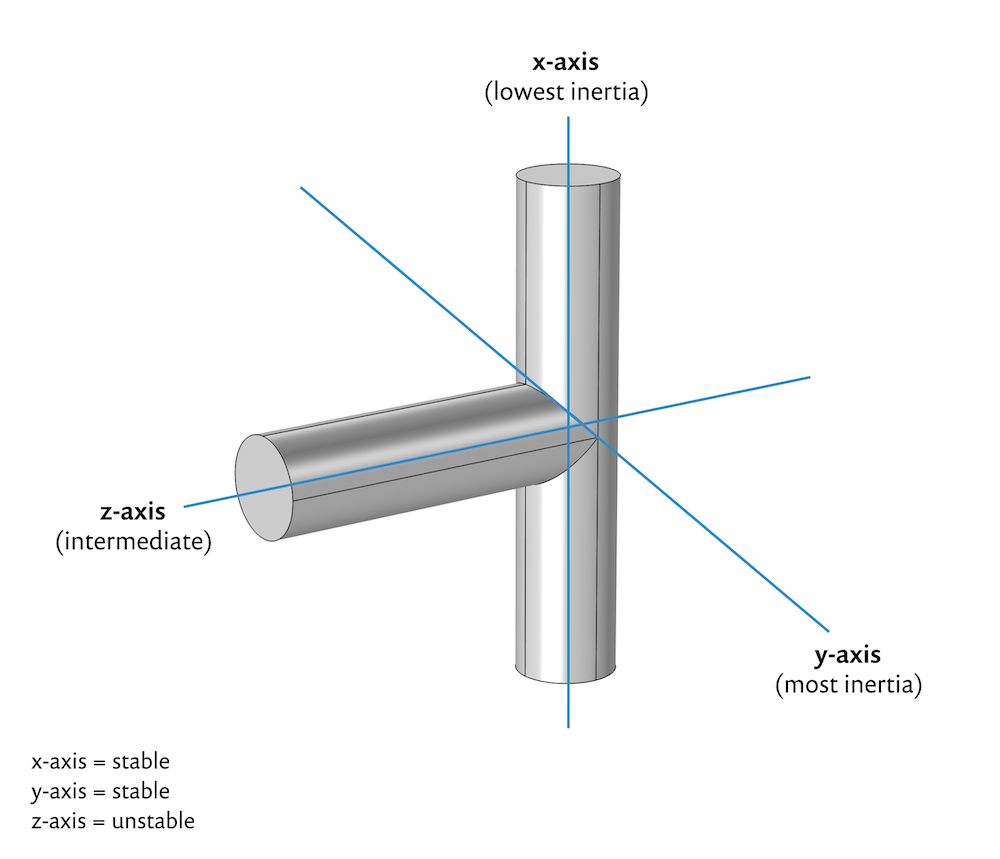
Vladimir Dzhanibekov noticed a peculiar effect in a wingnut in space, illustrated here using a simplified geometry.
This effect is not magic. It’s math.
For a three-dimensional body, it is possible to identify three special rotational axes. These axes have the property that when the body rotates about one of them at a certain angular velocity, the angular momentum of the body is given by the product of the angular velocity and the moment of inertia corresponding to this rotational axis. These moments of inertia are called principal moments of inertia, and the rotational axes are called principal axes of rotation.
For some bodies, the principal axes of rotation are easily identified, such as for the simplified wingnut geometry above, and for common objects like cereal boxes and cellphones.
What do wingnuts have to do with tennis rackets?
The Dzhanibekov effect is also called the intermediate axis theorem or tennis racket theorem. Tennis rackets also have three easily identified principal axes of rotation, so they exhibit the same behavior as wingnuts.
After Dzhanibekov noticed the phenomenon back in the 1980s, it was kept secret for years. However, a team of mathematicians independently noticed the effect in a tennis racket and elucidated the math behind it. They published their paper, “The Twisting Tennis Racket”, six years later.
The history of this effect’s complicated discovery is why the intermediate axis theorem goes by these two other names. Now that we know what it’s called and where it came from, how does this phenomenon work?
Euler’s Laws of Motion
The rotation of rigid bodies are described by Euler’s laws of motion. These laws are an extension of Newton’s laws, and extends them from Newton’s point particles to rigid bodies (like your cellphone or a cereal box). Euler’s equations are shown below:
Here, I_i is the principal moment of inertia along each of the three axes, \omega_i is the component of angular velocity along the axes, and M_i is the torque.
The value for the moment of inertia tells you how much torque you need to produce an angular acceleration about that axis (in other words, to make it spin faster or slower). The highest moment of inertia needs the most torque, while the lowest moment needs the least torque.
If we consider the case where a rigid body is rotating freely around the 3-axis, we can examine under what conditions this rotation is stable or unstable. This is done by assuming small perturbations to the angular velocities around the 1- and 2-axes. After some manipulations of Euler’s equations, we arrive at the following equation:
The part within the brackets is just a constant (let’s call it k). The constant will be either positive or negative depending on the values of the principal moments of inertia. If I_3 is greater than I_1 and I_2 (meaning I_3 is the largest moment of inertia), then (I_3 – I_2) and (I_3 – I_1) are both positive, and so k becomes positive. The same thing occurs if I_3 is less than both I_1 and I_2 (meaning I_3 is the smallest moment of inertia). Then, (I_3 – I_2) and (I_3 – I_1) are both negative, and again k becomes positive.
We get:
Look familiar? This is the equation for simple harmonic motion, because -k<0. This is a stable motion, meaning that a small perturbation will not bring the body out of its equilibrium.
What if I_3 is not the largest or smallest moment of inertia? For example, consider the case where I_3 is greater than I_2, but less than I_1. Then, k becomes negative. When the negative sign out front is included, we get a positive constant overall because -k>0. This equation is unstable.
In other words, the object’s stability is walking on the edge of a knife: Any force whatsoever, no matter how small, will cause it to tumble.
Multibody Analysis of an Object Displaying the Intermediate Axis Theorem
You don’t need to be in space to see this phenomenon in action. You can perform a multibody analysis using the COMSOL Multiphysics® software to explore the Dzhanibekov effect.
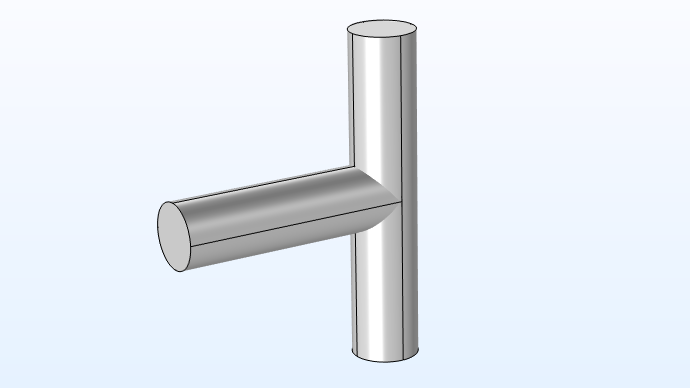
Consider an aluminum T-bar made up of two aluminum cylinders that have a 1 cm radius and height of 7 cm for the z-axis and 10 cm for the x-axis, as shown below.
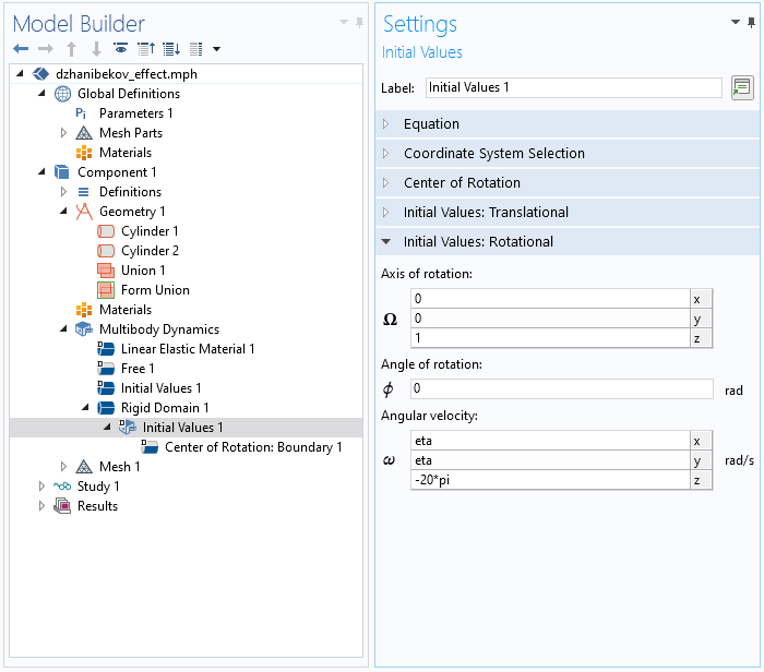
Using the Multibody Dynamics Module, an add-on to COMSOL Multiphysics, we can add a Rigid Domain boundary condition and select domains to make them a rigid body, as well as select the density as From material.
Editor’s note on 12/13/22: In version 6.1, the Rigid Domain feature has been renamed to Rigid Material.

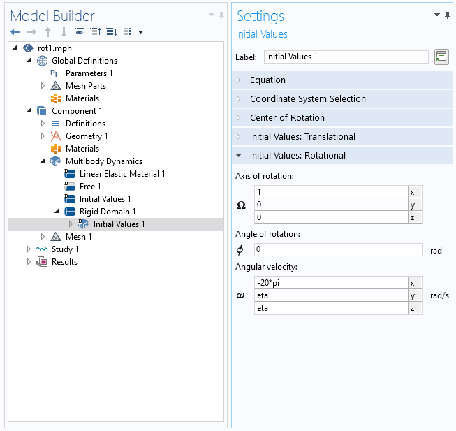
We can set the model to rotate on the z-axis as well as the following values for the axis of rotation and angular velocity:
The simulation illustrates how the end of the T-bar moves so that we can analyze its position or displacement with time.
You can alter or add different values to see how they affect the stability of the T-bar, such as changing the axis of rotation and angular velocity.
| x-axis | y-axis | z-axis |
|---|---|---|
|
|
|
|
The T-bar when rotating on the x-, y-, and z-axes.
By adding a point to the end of the T-handle, we can visualize the effect a lot more easily. This also lets us visualize the displacement of the T-handle from the main axis of rotation by plotting the displacement magnitude using the expression sqrt(u2+v2). In the graph below, the quantity is zero when the end of the T-handle bar is properly aligned with the z-axis, and remains stable until it starts to flip. The graph makes it more apparent that there is a stable region between flippings.
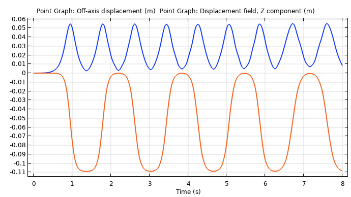
Blue line shows off-axis displacement (stable) and the orange line shows the displacement field, Z component (unstable).
To visualize this concept (and the 1D plot) even more, the animation below shows the displacement while the T-handle travels in an orbit about the z-axis, which you can show using a Point Trajectories plot. You can see that when the model becomes unstable, the orbit becomes larger and soon stabilizes when the point reaches the other end (this keeps repeating over and over again).
Taking the Dzhanibekov Effect a Step Further with a Simulation App
COMSOL Multiphysics includes the Application Builder, which enables you to transform a numerical model into an intuitive UI with specialized inputs and outputs. As an example, we built an app of the T-bar model shown above.
A screen recording of the Dzhanibekov Effect app.
You can use this app to test:
- 3 different geometries
- Original T-bar geometry
- Tennis racket
- Cellphone
- Axis of rotation
- X
- Y
- Z
Note: The cellphone and tennis racket geometries are unstable on the x-axis, whereas the T-bar is unstable on the z-axis.
You can also use the app to play the animation of the selected geometry and axis.
If you want to try demonstrating this effect in real life, we at COMSOL don’t take responsibility for any damage to your cellphone or tennis racket. In fact, using the app is probably a safer bet!
Next Step
Download the demo app, pick one of the geometries, choose which axis to rotate it on, and see what happens:


Comments (2)
Sergei Turovets
July 21, 2021Is the movement of a wingnut chaotic in the strict terms of dynamical chaos, i.e. the trajectories have a positive Lyapunov
exponent as in the Lorentz system ?
Pooja Pooja
May 16, 2024Call Girls In Gaur City Noida
If you’re looking for amazing and high-quality young women escort services in Gaur City Greater Noida West, if you have a picture of a gorgeous diva in your arms, and if you think that someone might be able to fulfil your fantasies, then contact The Gautam Buddh Nagar Hot Collection, who can arrange a call girl from Gaur City Noida Extension inside your room.
https://www.citycallgirls.in/call-girl-escort-services-in-gaur-city-noida/