

Previously on the blog, we introduced you to Linear Extrusion operators and demonstrated their use in mapping variables between a source and a destination. This approach, as explained earlier, is limited to cases in which the source and destination are related by affine transformations. Today, we will discuss General Extrusion operators, which are designed to handle nonlinear mappings and the mapping of variables between geometric entities of different dimensions.
A Short Recap of Extrusion Operators
At a point P_d in the destination entity, we want to compute a quantity that is a function of another quantity defined at the source entity. Thus, the latter quantity from a source point P_s needs to be copied to the destination entity. Extrusion operators are used to identify which point in the source entity corresponds to a point in the destination entity. In other words, the operators define the point-to-point map.
If the mapping is affine, it is sufficient to know how some points in the source correspond to points in the destination entity. From such source-destination pairs, one can infer the general mapping from superposition. However, in general, we need to write the mathematical expression for the mapping. This can be either an explicit definition of the source point P_s as a function of P_d or an implicit relation between P_d and P_s.
Using General Extrusion Operators in COMSOL Multiphysics
When using Linear Extrusion operators, we visually indicate the mappings for enough points (bases) and COMSOL Multiphysics figures out how to transform the remaining points. In the case of General Extrusion operators, we write out the mathematical description of the mapping for an arbitrary point in the destination.
To begin, let’s focus on how to replicate a Linear Extrusion operator with a General Extrusion operator. We can then consider examples in which the General Extrusion operator must be used.
For affine relations, General Extrusion operators can be used as an alternative to Linear Extrusion operators. When it comes to general nonlinear mappings, General Extrusion operators are necessary. To add a General Extrusion operator, we go to Definitions > Component Couplings > General Extrusion.
Example 1
In our earlier blog post on Linear Extrusion operators, we considered an affine mapping that pairs up points 1, 4, and 2 in the source domain to points 1, 5, and 3 in the destination domain. Take a look at the figure below. The two circles in the geometry have centers at the origin and radii of 1.0 and 1.5.
Any affine transformation can be expressed as the sum of a linear transformation and a translation operation. Therefore, we have
Now we need to find the constants a,b,c,d,e, and f. Since source points (0, 0); (1.0, 0); and (0, 1.0) correspond respectively to destination points at (0, 0); (1.5, 0); and (0, 1.5), we get
Now that we know how to find the corresponding coordinates of the source point, given any point (x,y) in the destination, we enter the right-hand side of the above equation (without the subscripts) in the destination map of the General Extrusion settings window.
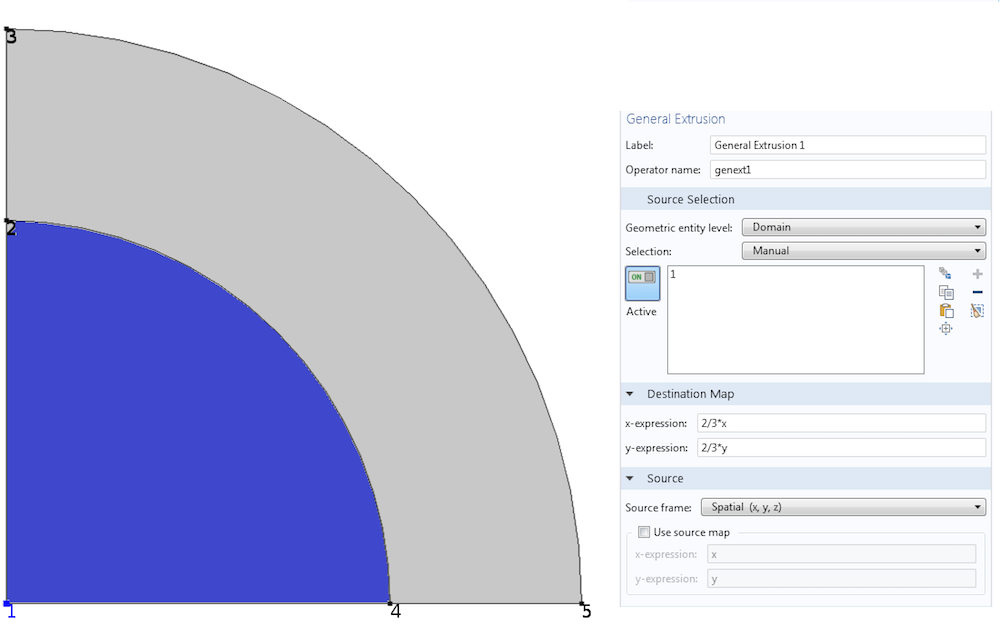
A linear mapping built using a General Extrusion operator.
Example 2
Let’s now explore how to use a General Extrusion operator to copy data from a 2D axisymmetric component to a 3D component, such that the source and destination points correspond to the same point in space. Consider thermal expansion with axisymmetric thermal boundary conditions and material properties. If the structural boundary conditions are not axisymmetric, we can save time by performing an axisymmetric thermal analysis in one component, and then mapping the temperature from the 2D axisymmetric domain to the 3D domain for structural analysis in another component.
When building the mapping, it is important to ask the following question: Given the coordinates of the destination point, how do we go to the source point? In this instance, that relationship is given by
As in Example 1, we enter the expression on the right-hand side in the destination map.

Using a General Extrusion operator to copy data from the 2D axisymmetric domain to the corresponding 3D domain. Note that for axisymmetric components, variables can be viewed in 3D with a Revolution 2D data set in the Results node. However, if we want to use variables from a 2D axisymmetric component in the physics node of a 3D component (i.e., thermal expansion), we need to utilize General Extrusion operators.
The operator genext1 is not known inside the 3D component comp2; neither is T. If we want to use the temperature from the 2D axisymmetric component as an input in the 3D component, we have to use comp1.genext1(comp1.T). This approach helps avoid confusion if there is an extrusion or another operator also called genext1 or another variable called T in the second component.
Note that a Linear Extrusion operator cannot be used here. Because the source and destination objects have different dimensions, affine transformations are impossible.
In these first two examples, the Use source map check box in the Source section of the settings window has been left unchecked. COMSOL Multiphysics filled in x and y in the first case and r and z in the second case. When this check box is left unchecked, COMSOL Multiphysics assumes that we have explicit expressions for each coordinate of the source as functions of coordinates of the destination. Oftentimes, however, we may not have explicit expressions.
Next, we’ll look at how to use a General Extrusion operator to specify implicit relations.
Example 3
A 2D parabolic curve given by \frac{y}{d} =(\frac{ x}{d})^2 is in a square domain of side d. Our task is to build an operator that maps data from this curve (represented in blue in the figure below) to different parts of the square. The parabola is the source. We want an operator that will copy from a point on the parabola to a point in the square, such that the distance of the destination point from the origin is equal to the length of the segment of the parabola between the origin and the source point.
A little calculus gives us the arc length of the parabola between the origin and the source point (x,y).
The relationship between the source and destination points is therefore
If we want an explicit source-destination mapping of the form
we first need to invert the expression L=\frac{x_s}{2}\sqrt{1+4(\frac{x_s}{d})^2}+\frac{d}{4}\ln(2\frac{x_s}{d}+\sqrt{1+4(\frac{x_s}{d})^2}) and write x_s in terms of L. That’s no fun at all!
This is exactly why COMSOL Multiphysics allows us to specify implicit relations between source and destination coordinates by using two mappings: the destination map and the source map. We need to provide T_d and T_s, such that

Using source and destination maps to define implicit relations between source and destination coordinates in a General Extrusion operator.
COMSOL Multiphysics will take care of T_s^{-1}(T_d(x_d,y_d)), a necessary step in identifying the source coordinates. Note that the source map needs to be one-to-one for the inverse to exist. In practice, COMSOL Multiphysics does not construct an analytic expression for the inverse of the source map. Instead, at every destination point, it first evaluates T_d(x_d,y_d) and carries out a mesh search operation to find the point on the source where this evaluation matches T_s(x_s,y_s). A one-to-one source map makes the search return, at most, one source point for a given destination point.
In the General Extrusion settings window shown above, the labels under Destination Map and Source read x^i–expression and y^i–expression rather than x–expression and y–expression. The reason is that x^i and y^i are indices for the first and second pairs of expressions used to define the source-destination relationship implicitly. They are not necessarily pertaining to the x or y coordinates in the source or destination. These indices are, in a sense, coordinates of an intermediate mesh, and a General Extrusion operator matches source and destination points that have the same intermediate coordinates. In this example, one expression is sufficient enough to uniquely relate any destination point in the square domain to a source point on the parabolic curve. Thus, the second line y^i–expression is left blank.
To see how this General Extrusion operator maps variables, consider a plane stationary heat conduction problem with the left and right edges at temperatures of 300 K and 400 K, respectively. The top and bottom surfaces are thermally insulated, and there are no heat sources. The temperature will vary linearly with x. From the graph below, can you see why the plot of arcext(T) on the right shows a radial variation?
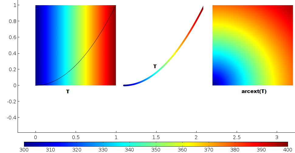
Left: Temperature varies linearly from left to right. Center: Temperature along the parabola. Right: Temperature mapped from the parabola to the domain. All points in the domain with the same distance from the origin copy temperature from the same point on the parabola.
Piecing Everything Together
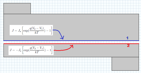
To apply what we have learned thus far, let’s now build a diode model using the Electric Currents physics interface in COMSOL Multiphysics. Extrusion operators help us construct normal current density boundary conditions on each side of the ideal p-n junction. We can tag the different sides as 1 and 2, as illustrated in the figure below. The Shockley diode equation for the current-voltage (I-V) relation is used at the junction. The parameters J_s, q, k, \textrm{and } T represent the following, respectively: the saturation current density, the electronic charge, Boltzmann’s constant, and temperature.
Extrusion operators can be used to access the electric potential on the other side of a junction.
To implement the normal current boundary condition on side 1, we need access to the electric potential V_2 on side 2. Similarly, on side 2, we need access to the electric potential V_1 on the other side of the junction. Thus, two extrusion operators are required. Each side of the junction becomes a source entity in one of the extrusion operators, as depicted below.


Both cases involve mapping between points that share the same x-coordinate. Because the source entities are different, two operators are needed.
Now we will use the operators in the physics nodes to implement the boundary conditions. The boundary condition at the top side is illustrated below. Note that V refers to the electric potential at a point on the top side while genext2(V) refers to the electric potential vertically on the bottom side.

Using a General Extrusion operator to refer to the electric potential at a point on the other side of the junction.
A similar boundary condition is used on the bottom side of the junction. The corresponding normal current density for the Normal Current Density 2 node applied to edge 3 is -Js*(exp((V-genext1(V))/kTbyq)-1). Here, V refers to the electric potential at a point on the bottom side, while genext1(V) refers to the electric potential vertically on the top side.
In fact, a shortcut can be made by using the expression genext2(V)-genext1(V) for the voltage difference, regardless of which side it is being applied. For clarity, we did not use this trick here.
With a voltage terminal at the bottom of the device and ground at the top of the device, the following results are obtained.
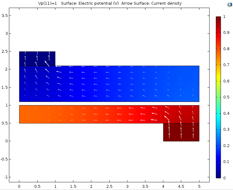
Extrusion operators can be used to make couplings between points in the same component or different components. Here, the p-n junction in a diode is represented by a thin gap in the geometry. The electric potential on one side of the gap is accessed from the other side by using an extrusion operator in order to compute the current density flowing across the gap.
Other Component Coupling Operators
Extrusion operators are used to construct pointwise relations between source and destination points. Sometimes, we may want to access an integral, average, maximum, or minimum over a source line, surface, or volume. In such cases, we can use projection, integration, average, maximum, or minimum component couplings. You can learn more about the use of projection operators in this previous blog post.
Closing Remarks
Today, we have discussed how to use General Extrusion operators to create mappings for copying variables from one part of a simulation domain to another. In addition to simply copying known quantities, these operators can be used to create nonlocal couplings between unknown variables, as illustrated in our p-n junction example. This approach is also useful in other analyses including structural contact or surface-to-surface radiation in heat transfer. COMSOL Multiphysics includes built-in features pertaining to such physical effects.
If the nonlocal couplings you want to simulate are not included in the built-in features of COMSOL Multiphysics, you can use the strategies you’ve learned today to implement them. Please feel free to contact us if you have any questions!
Further Reading
To explore the use of General Extrusion operators in other types of situations, consult the following blog posts:


Comments (2)
Kudakwashe Chayambuka
February 4, 2016Thank you so much for this article, I was in need of something that shows the mathematical operations of the extrusion coupling
Carl Weggel
June 9, 2020I deplore the glaring oversight of COMSOL: Considering how frequently one encounters problems that include a combination of Rotationally-Symmetric and Cartesian components, that COMSOL has not seen fit to provide a specific operator for this case!