

Sweeps are very useful for characterizing a system and learning more about how different input values impact the results. You can perform several different types of sweeps in the COMSOL Multiphysics® software, including function, material, and parametric sweeps. However, precise and innovative simulation results also call for mathematical optimization. In this blog post, learn how to combine sweep studies with the built-in optimization functionality.
Achieving the Ideal Frequency of a Tuning Fork
Tuning forks are made out many different materials, but most of them are calibrated to a standard pitch of 440 Hz for an A note. An article in JOM discusses how the frequency of a tuning fork changes with different materials and a fixed geometry (Ref. 1). This made me think: What if we change the geometry and material of a tuning fork to reach the desired frequency?
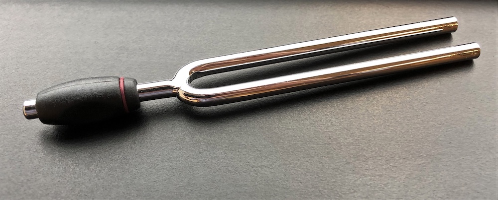
A tuning fork.
Performing an Optimization Study for Multiple Materials
The Application Library contains several models featuring a tuning fork geometry, as well as a tuning fork simulation app. You can access the Application Library within the COMSOL® software GUI in the File menu and search the keyword “tuning fork”. For this blog post, we’ll start with the simple Tuning Fork model (and accompanying example app).
This model features a parametric geometry, material properties of steel, the Solid Mechanics interface, and two studies. Both studies perform an eigenfrequency analysis to search for the eigenfrequency around 440 Hz. The first study uses a parametric sweep of the tuning fork’s arm length, set as a parameter L, to find the optimal design for 440 Hz. In contrast, the second study applies a mathematical optimization algorithm that uses L as the control variable and the deviation from the target frequency as the optimization objective for fast, precise, and efficient optimization.

Tuning Fork model showing the original settings to search for a tune of 440 Hz via two different strategies.
Let’s return to the initial question: How does the tuning fork’s arm length depend on the material for a tune of 440 Hz?
First, we extend the model with a material switch. This option allows us to set and test various materials for the model. Further, this switch is needed to work with the material sweep in the Study node, as described later in this blog post. We can add available materials from the built-in Material Library, including:
- Aluminum
- Titanium beta-21S
- Copper
- Steel AISI 4340
The switch is assigned to the solid domains of the tuning fork.
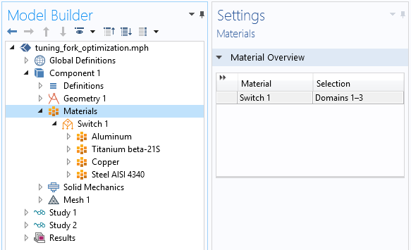
Setting the material switch for a multimaterial analysis.
Now that we transformed the original model into a multimaterial model, we can adjust the studies. Due to the combination with a material sweep, the studies can now solve the physical model for all chosen materials and it is possible to analyze all of the results together. For example, we can look at the eigenfrequency and confirm that the eigenfrequency changes with different materials and arm lengths.
Various sweeps can be combined easily within a study, such as the extension of Study 1 with a material sweep. In contrast, when we try to add a material sweep to the optimization study for Study 2, we get an error message. The good news is that there is another way of achieving this by using Study References, as explained below.
Setting the material sweep directly in the study is not supported, since it is only possible to use one Sensitivity, Optimization, Parameter Estimation, or Parametric/Material/Function Sweep study step in each study. These study nodes tend to control the same solver settings and are therefore incompatible with each other. To perform a parametric or nested optimization, we can call a study containing an Optimization node from inside another study via a Study Reference node.
Therefore, we add an additional empty study and fill it with a Material Sweep node and a study reference pointing to the optimization study. In the Optimization node, we can define the settings needed for the optimization. This is possible as long as all entries are globally available. For that, we leave Study 2 containing the optimization as is.
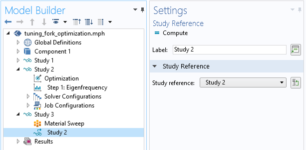
Use of an additional study to create nested studies.
Optimizing a Tuning Fork for Various Materials in COMSOL Multiphysics
With all the discussed adjustments, we can now run the multimaterial optimization study by computing Study 3. This study controls the material assignment and runs individual optimization procedures for each by starting Study 2 automatically. Hence, we can extract and postprocess the individual design changes for the different materials. This can be done, for example, by a global evaluation of the parametric data set. Evaluating the tuning fork arm length, set as the control variable L, gives us the needed design changes to tune each tuning fork design to 440 Hz.
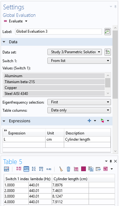
Top: Settings of the global evaluation. Bottom: Results table for the different materials identified via the switch index.
Testing Tuning Fork Design Parameters with an App
You can build an app from a tuning fork model that includes a customized user interface and restricted inputs and outputs. Take the Tuning Fork app in the Application Library as an example. This app can be used to quickly compute the frequency of a tuning fork with the prong length as an input or the optimal prong length with the frequency as an input.
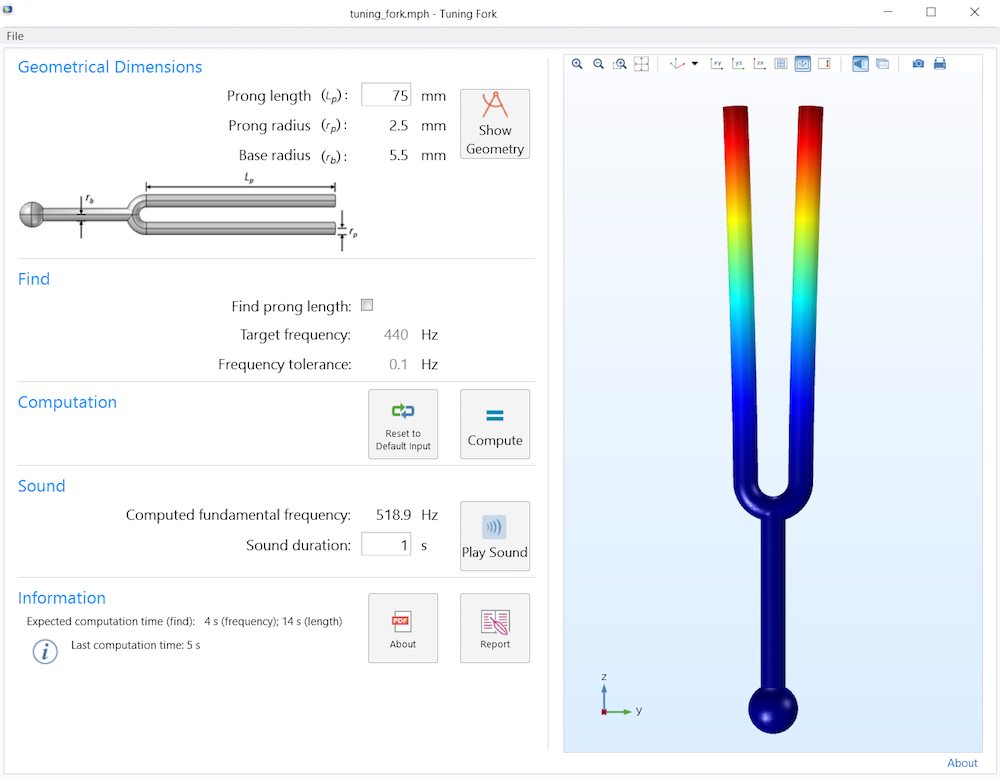
The user interface of an example tuning fork app.
The example featured above can be used as inspiration for building apps of your own via the Application Builder tool in COMSOL Multiphysics.
Concluding Thoughts on Multimaterial Optimization
In this blog post, we used material sweeps in combination with an optimization study to find the best geometry for tuning forks made of different materials. Note that the approach discussed here is generic. You might want to combine other study steps that have the same hierarchy.
With this approach, you can combine all of the Sensitivity, Optimization, Parameter Estimation, or Parametric/Material/Function Sweep features into nested studies, thus improving your simulations, results, and products.
Next Steps
Try it yourself: Access the Tuning Fork model and app by clicking the button below, which will take you to the Application Gallery.
Read More on the COMSOL Blog
Reference
- T.D. Burleigh and P.A. Fuierer, “Tuning Forks for Vibrant Teaching“, JOM, pp. 26–27, Nov. 2005.


Comments (2)
Ivar KJELBERG
April 4, 2018Hi Friederich
Thanks for an illustrative Blog.
I believe we can study far more with the tuning fork, as today COMSOL Multiphysics(r) Blogs and Application models show us how to optimise the tuning fork, but does not really tell us why a tuning fork is only oscillating on the pure 440 Hz line and not on some of the other eigenmodes.
This you may also nicely illustrate by pushing your model slightly further:
here are some hints for a nice blog you could get to illustrate the interesting features you can now extract with your FEM tool, thanks to the implementation of the detailed modal mass and inertia participation factors, and COMSOL Multiphysics(r) nice way to give us access to the true complex eigenvalues.
On the proposed Application model:
– add a new Eigenfrequency study,
– add a parametric sweep and set the L value to the optimised one of the first study,
– then ask for the first 12 modes (and not only the default first 6, or the unique one as in your example).
Then to illustrate the way one holds a tuning fork:
– add to the model a spring/damper link,
– select the end ball boundaries {11-16, 18, 20} and
– set a spring constant of some 1E6 N/(m*m^3) and
– a loss factor of scalar-type of some 0.8 .
You may play with these values as they drive heavily the first eigenmode values of the tuning fork, and represents the way your finger hold actually a true tuning fork, with some stiffness and quite some damping.
The result is a set of complex modes, except for the 440 Hz mode that show up clean and “real”.
This can be further pushed by dumping all the 6 mass and inertia modal participation factors:
– add the “Definition – Variable Utilities – Participation Factors” node before you solve.
The first 6 modes below 440 Hz that have large imaginary eigenfrequency parts, hence are strongly damped, and also have all “large” absolute participation factors, at least compared to the one at 440 Hz :
Main reason:
this 440 Hz mode is a symmetric mode in each fork branch, leaving the CoG of the vibrating fork at its central location, hence show up as a “0” participation factor items, EVEN if it is the mode with the most “energy” and vibrating the most. This illustrates well how tricky it is to look only on mass participation factors! One need to add quite some “engineering sense” too. All these first modes make your finger touch to vibrate and then be damped by the fingers, but NOT the symmetric 440Hz mode!
Depending on the damping factor and spring stiffness used the higher eigenmodes above the 440 Hz one might also have complex eigenfrequencies, indicating noticeable damping.
So when one hit the tuning fork, held in your hand, the hand and the system “fingers-tuning fork” are the filtering system that ensures the correct tone, and adapting the grip you might manage to keep one or some of the overtones for shorter or longer period.
So the tuning fork example is a nice example to explain and illustrate further the effect of:
– damping,
– complex eigenfrequencies,
– participation factors,
and how a small change in the “fixed” BC’s might completely change your problem and solutions.
Thanks again for an illustrative Blog
And let’s continue to have fun COMSOLing
Sincerely,
Ivar
Bjorn Sjodin
April 4, 2018Hi Ivar,
Thanks for your comment. Indeed, we are already working on one or more blog posts with regards to tuning forks and we will take your comments in consideration. It seems tuning forks is a great source of blog material for structural dynamics.
Bjorn