

Have you ever been curious about how to model supersonic flows, like those around Concorde or fighter jets? Generally, this process requires the resolution of shocks or expansion fans in the flow. Resolving discontinuities (e.g., shock waves) requires a high resolution and the numerical stability of strongly coupled mass, momentum, and energy conservation equations for fluid flow. Let’s discuss how to model supersonic flow past a diamond airfoil, which involves resolving shocks and expansion fans.
What Is the Difference Between Subsonic, Sonic, and Supersonic Flow?
Consider a wing moving in air, say at a constant speed u. The disturbances created by the wing propagate as pressure waves in air (here, sound waves), so these disturbances propagate at the local speed of sound, a. If the speed of the wing is smaller than the speed of sound, u < a, the disturbances propagate faster than the wing itself. Therefore, the fluid upstream is influenced by the presence of the wing before the wing reaches that location. As the speed of the wing is below the speed of sound, this is known as subsonic flow. This phenomenon can also be represented in terms of the Mach number, Ma = u/a 1), the fluid upstream is no longer influenced by the wing before it reaches that location, since the pressure waves have not propagated there yet, as shown in the image below (Mach cone in red). The disturbance propagation gives us qualitative insight into the demarcation between the subsonic and supersonic flow regimes.
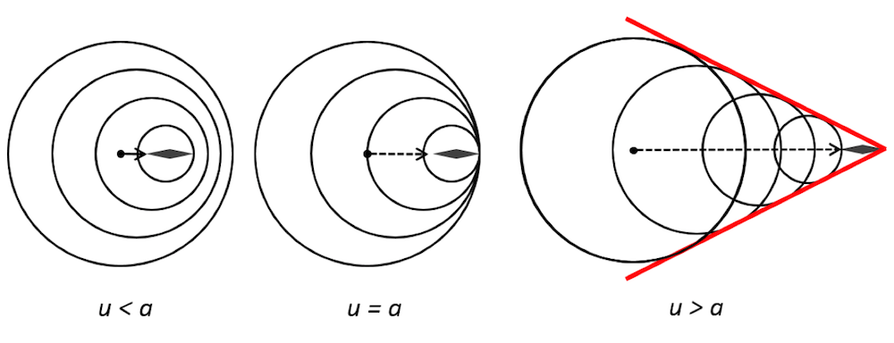
The disturbance propagation for subsonic (left), sonic (middle), and supersonic (right) wing speeds, where the circles represent the pressure/sound waves. The arrow represents the direction of movement of the object.
To quantitatively resolve the fluid flow, we first determine whether the flow will be in the laminar flow regime or if it will have transitioned into a turbulent flow regime. The flow regime is based on the Reynolds number, Re = ρuL/μ. Here, ρ, μ, and u are the fluid density, dynamic viscosity, and speed, respectively. The characteristic length (the chord length in the case of a wing) is denoted by L. We then solve either the Navier-Stokes equations with continuity and constitutive relations for laminar flow or the Reynolds-averaged Navier-Stokes equations with continuity and constitutive relations for turbulent flow. Depending on the problem, a suitable turbulence model can be used to resolve the turbulence.
If the flow becomes highly compressible, as is the case for supersonic flows, the energy equation has to be solved in addition to the mass and momentum conservation equations mentioned earlier, whether the flow is in the laminar or turbulent flow regime. The viscous effects in supersonic flows are usually negligible, except in the regions with sharp gradients such as shocks or boundary layers. However, if the viscous effects in the regions of interest are negligible, then removing the viscous terms in the Navier-Stokes equations yields the Euler equations. These inviscid flow equations can be solved analytically for simple geometries.
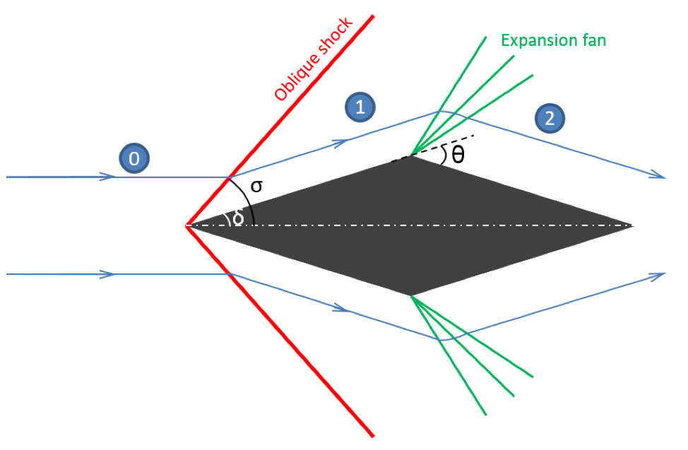
The supersonic flow field around a diamond airfoil, showing the different regions in the flow field.
For simplicity, consider the benchmark case of supersonic flow past the cross section of a wing with a diamond airfoil. This topic has already been investigated by COMSOL Multiphysics® users in the paper “Numerical Study of Navier-Stokes Equations in Supersonic Flow over a Double Wedge Airfoil using Adaptive Grids“. As mentioned earlier, the fluid upstream (zone 0 in the figure above) is not influenced by the disturbances caused by the airfoil. So when the fluid approaches the airfoil, it faces an abrupt decrease in flow area (similar to a concave corner) and has to suddenly change its direction to match the boundary conditions in zone 1.
This process can only occur if there is a discontinuity in the flow. This discontinuity is known as a shock wave and is very thin; i.e., on the order of the mean free path of the gas molecules, which is around 50 nm in air at atmospheric pressure. When a shock wave is inclined to the flow direction due to the shape of the object and the flow’s Mach number, it is called an oblique shock wave. Across a shock, the static pressure, temperature, and density increase, while the Mach number and total pressure decrease.
Calculating the Shock Angle and Mach Number of a Shock Wave
As mentioned above, when we assume inviscid flow (which is usually a valid assumption to estimate flow properties in supersonic flows), the shock angle (σ) can be determined for a weak shock based on the inclination of the object. Here, this is the half angle of the diamond airfoil (δ) and the upstream Mach number (Ma0).
For a fluid with specific heat ratio γ, the Mach number after the oblique shock in zone 1 can be estimated from:
After the shock along the diamond airfoil, the flow encounters an expanding area around the top of the airfoil (similar to a convex corner). The change in the flow direction to match the boundary conditions is achieved through an expansion fan, also known as a Prandtl-Meyer expansion fan. Across an expansion fan, the static pressure, temperature, and density decrease, while the Mach number increases. Again, by assuming inviscid flow, we can estimate the Mach number after the expansion fan based on Ma1 and the turning angle (θ) from:
Based on the above equations, we can estimate the shock angle and the Mach number across a shock wave or expansion fan. Similar estimates for pressure, density, and temperature can also be computed. However, for more complicated geometries where the shock/expansion waves interact or for highly viscous fluids, it would be more appropriate to resolve the flow through the numerical solution of the conservation equations in their entirety. Let’s model this simple benchmark case of a diamond airfoil and compare the results with estimates from the above equations.
Modeling Supersonic Flow Past a Diamond Airfoil in COMSOL Multiphysics®
As mentioned earlier, the flow in this scenario becomes highly compressible at supersonic speeds, which leads to a strong coupling of all of the conservation equations. These equations now have to be solved together to resolve the shock waves and the expansion fans that occur in the flow field, which can be done using the High Mach Number Flow interface in the CFD Module. Let’s take a look at how to set up a model of supersonic flow past a diamond airfoil using the High Mach Number Flow interface.
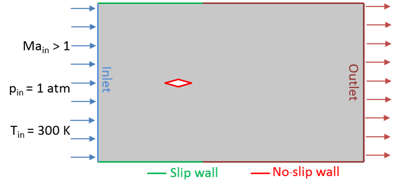
The model configuration, including the boundary conditions.
A schematic of the model setup, along with the static pressure and temperature at the inlet, is shown above. Based on the inlet conditions and airfoil chord length, the Reynolds number is found to be greater than 3 x 10⁵, indicating that the flow is in the turbulent regime. Therefore, the k-ε turbulence model is used here.
A hybrid flow condition is used under the outlet boundary condition. This condition allows for the flow at that boundary to be either supersonic or subsonic. If the flow is subsonic, then the static pressure specified under the condition’s settings would be ensured. A no-slip condition is defined on the airfoil and a combination of slip wall and outlet (hybrid flow) boundary conditions are used on the top and bottom walls to mimic the inviscid model equations that are solved analytically. In addition, since this is definitely a nonlinear problem, it is important to note that we can achieve better convergence for the problem by specifying initial conditions that could be close to the final solution — as discussed in a previous blog post on nonlinear static finite element problems.
As mentioned earlier, a shock wave is a form of discontinuity in the flow field. Therefore, a very fine mesh must be used at and around the pressure wave in order to numerically resolve this region. The spatial location of the shocks or expansion fans is not known ahead of time. In addition, we might be interested in computing the flow field for varying angles of attack and different inlet conditions, which would result in different locations of shocks in the domain. Therefore, if a uniform mesh is used for such problems, it would need to have a very high mesh density everywhere, significantly increasing the computational cost. However, in the COMSOL Multiphysics® software, we can take advantage of adaptive mesh refinement (an option available in the solvers) to dynamically adjust the mesh refinement in the domain, such that a fine mesh is created near the discontinuities and a comparatively coarser mesh is used in the remaining domain. Here, the conditions for adaptive mesh refinement are defined under the settings for the Stationary study step.
The results from the study and those from the expressions given in the previous section are listed in the table below for comparison. The results from COMSOL Multiphysics are evaluated in the midsection of the zones along the streamline, shown in the streamline plot below. The simulation results and theoretical estimates are within 3% of each other, as indicated by the tabulated results. It is also important to note that any viscous effects present in the problem are taken into account by the numerical model, making it more physically accurate than the inviscid theory on which the analytical estimates are based.
| Zone Number | Mach Number (Theory) | Mach Number (Model) | Static Pressure (atm) (Theory) | Static Pressure (atm) (Model) | Static Temperature (K) (Theory) | Static Temperature (K) (Model) |
|---|---|---|---|---|---|---|
| 0 | 2.0 | 2.0 | 1.0 | 1.0 | 300 | 300 |
| 1 | 1.45 | 1.44 | 2.22 | 2.21 | 378 | 381 |
| 2 | 2.55 | 2.53 | 0.40 | 0.41 | 231 | 237 |
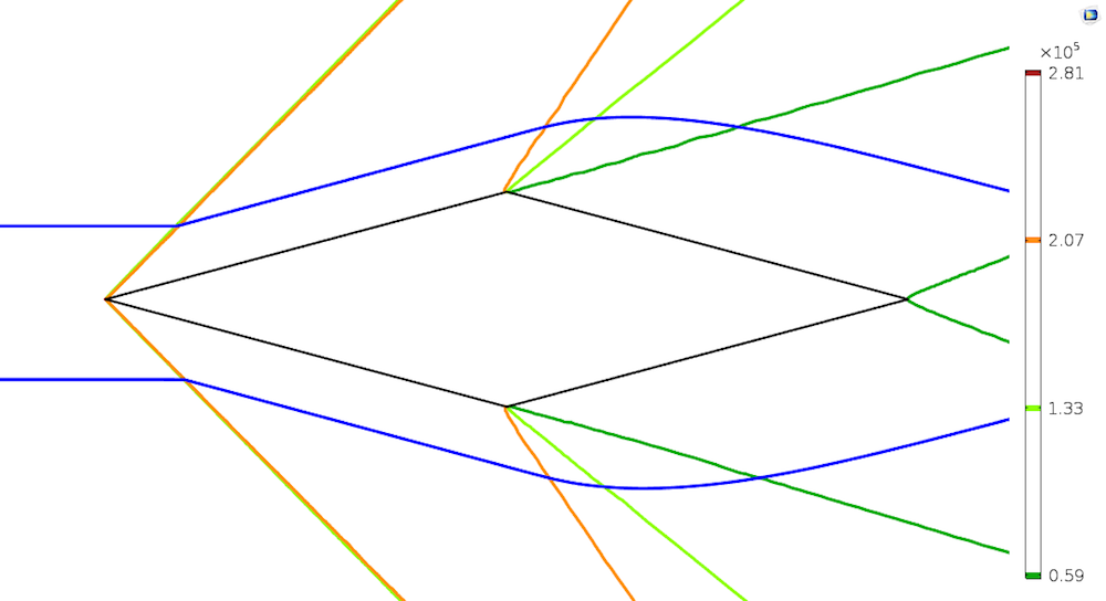
A contour plot of the static pressure (in Pa) along with the streamlines (in blue) for zero angle of attack, an inlet Mach number of 2.0, pressure of 1 atm, and temperature of 300 K.
A comparison of the shock angle is qualitatively shown in the Mach number surface plot below. At the location of the shock, a sudden change in the Mach number is observed. In the following plot, a black line has been added to indicate where the shock would be located based on the theoretical estimates. There is good agreement between the theoretical estimates and the simulation results.
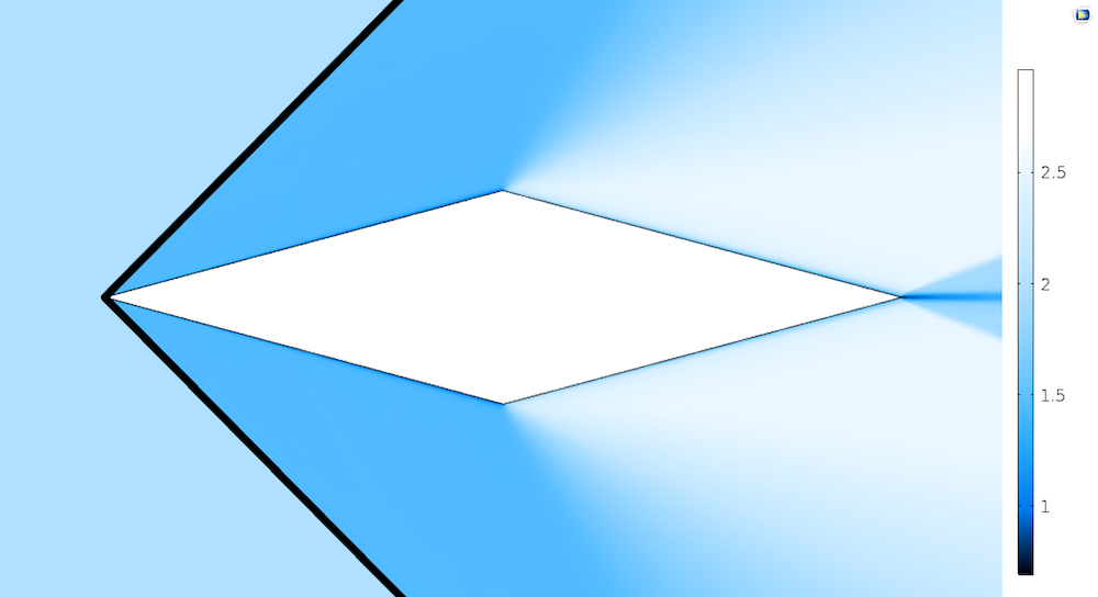
A surface plot of the Mach number. The black lines indicate the location of the shock based on expressions for shock angle, zero angle of attack, an inlet Mach number of 2.0, pressure of 1 atm, and temperature of 300 K.
Below, we can see the temperature surface plots for varying angles of attack. In addition to the temperature changes on the top and bottom sides of the airfoil, the change in the shock angle with the change in angle of attack can be clearly observed in these plots. At a 10° angle of attack, the angle of inclination at the bottom becomes 25° (as the half angle is 15°). The analytical theory predicts detachment of the shock, which is also observed in the numerical analysis (shown in the figure below on the right).

A surface plot of the temperature (in K) for varying angles of attack (α) for an inlet Mach number of 2.0, pressure of 1 atm, and temperature of 300 K.
Concluding Remarks
In this blog post, we have discussed supersonic flow characteristics such as shocks and expansion fans. With an example of supersonic flow over a diamond airfoil, we have shown how these characteristics can be resolved in COMSOL Multiphysics using the High Mach Number Flow interface. The shock angle and flow properties on the airfoil from our simulations are in good agreement with analytical estimates from inviscid compressible flow theory.
Further Resources
For more information on modeling supersonic or transonic flows, check out these example models from the Application Gallery:


Comments (6)
Md Farhadul Islam
March 5, 2018Very good post. Do you know how to detect shock through a CD nozzle using COMSOL?Is there any method for that ?
Siva Sashank Tholeti
March 6, 2018Hi Md Farhadul, the occurrence and location of shocks are detected while analyzing the results. When Mach number is plotted, a very sharp decrease in Mach number, as shown in the final plots in this blog, indicates the presence and location of a shock. This can be detected by plotting pressure and temperature as well.
The example “Transonic Flow in Sajben Diffuser” will help you with modeling and detecting shocks in a CD nozzle.
SPT Takti
March 17, 2020Hi Siva
Could you help me with acoustic analysing in CD nozzle at high mach number?
Is there any multi-physics that can relate hmnf to acoustic?
Siva Sashank Tholeti
March 18, 2020 COMSOL EmployeeHi SPT Takti, please contact support@comsol.com to help address this question. Thanks.
Ahmad Gad
December 24, 2021Thanks for the topic, Siva. I have a quick question.
Can the High Mach Flow Module solve a similar problem for water? And If I need to model a shock wave in COMSOL on fluids like water (assuming that they will change phase), which module shall I use? And Do I need to use a Thermodynamic Module along with it to identify the different phases of the material?
Thanks a lot, in advance.
Siva Sashank Tholeti
December 28, 2021 COMSOL EmployeeHi Ahmad, thanks for the question. The High Mach Number Flow physics interface assumes ideal gases and is limited by that assumption. However, ideally one could use a Laminar or Turbulent Flow interface coupled with Heat Transfer in Fluids to model highly compressible flows in fluids (in general), which might require careful set-up. Please contact support@comsol.com for information on this. Thanks.